Introduction to Simulation Based Inference

Introduction to Simulation Based Inference#

Having a simulator - a “black box” that can produce data under any model parameters - can prove very valuable because in some problems it is impractical or even impossible to write down a form of the likelihood.

A simulator can help sample from an untractable likelihood
This can prevent wrong result if a wrong likelihood is chosen
Perform Simulation-Based parameter inference using:
- Approximate Bayesian Computation, and
- Neural Posterior Estimation
How Normalizing Flows can create very expressive generative models to sample from

Disclaimer: This is probably the most demanding lecture of the school, containing multiple notions and tools that you learned in previous lectures and linking them in intricate ways.

Note: This notebook is shortened compared to the full version that can be found in the material of previous schools, where all the methods and more details can be found.

Setup#

# --- Compatibility patch for GetDist + NumPy 2.0 ---
# NumPy 2.0 removed np.infty, but older versions of GetDist still use it.
# This patch restores it at runtime before importing GetDist.

import numpy as np
if not hasattr(np, 'infty'):
    np.infty = np.inf  # Restore deprecated alias for compatibility

import torch
import torch.nn as nn
import torch.nn.functional as F
from torch.utils.data import TensorDataset, DataLoader, random_split
import numpy as np
import emcee
from scipy.stats import poisson
from scipy.stats import chi2
from scipy.optimize import basinhopping
from tqdm import tqdm
import matplotlib.pyplot as plt
import pytorch_lightning as pl
from scipy.stats import norm
from getdist import plots, MCSamples
from scipy.integrate import quad
import multiprocessing
from multiprocessing import Pool

from nflows.flows.base import Flow
from nflows.distributions.normal import StandardNormal
from nflows.transforms.base import CompositeTransform
from nflows.transforms.autoregressive import MaskedAffineAutoregressiveTransform
from nflows.transforms.permutations import ReversePermutation
from sbi.inference import SNPE
from sbi.utils.torchutils import BoxUniform

import requests
from IPython.display import display, HTML
display(HTML("<style>.container { width:100% !important; }</style>"))

url = "https://raw.githubusercontent.com/AstroStat-Academy/assets-public/main/colab/clone_and_cd_colab.py"
colab = requests.get(url).text
exec(colab)

url = "https://raw.githubusercontent.com/AstroStat-Academy/assets-public/main/styles/plot_style.py"
style = requests.get(url).text
exec(style)

%matplotlib inline

torch.__version__

Introduction#

Revisiting Bayesian Inference#

The goal of Bayesian inference is given some observed data $x$, to infer the distribution of the parameters $\theta$ of some model that is consistent with the data, i.e. the posterior distribution $p(\theta|x)$. This is achieved using Bayes’ theorem:

\[ \Large p(\theta|x) = \frac{p(x|\theta)p(\theta)}{p(x)}\]

Some examples from astronomy for the observed data $x$ and the model parameters $\theta$ are:

x	θ
observed X-ray photon count of a galaxy cluster	the mass of the cluster
gravitational wave signal from a collapsing black hole binary	the mass ratio and ellipticity of the binary
2D sky projection of galaxy weak lensing measurements	the cosmological parameters governing dark matter and dark energy
the distorted arcs of a strongly lensed galaxy	the mass distribution of the lensing galaxy

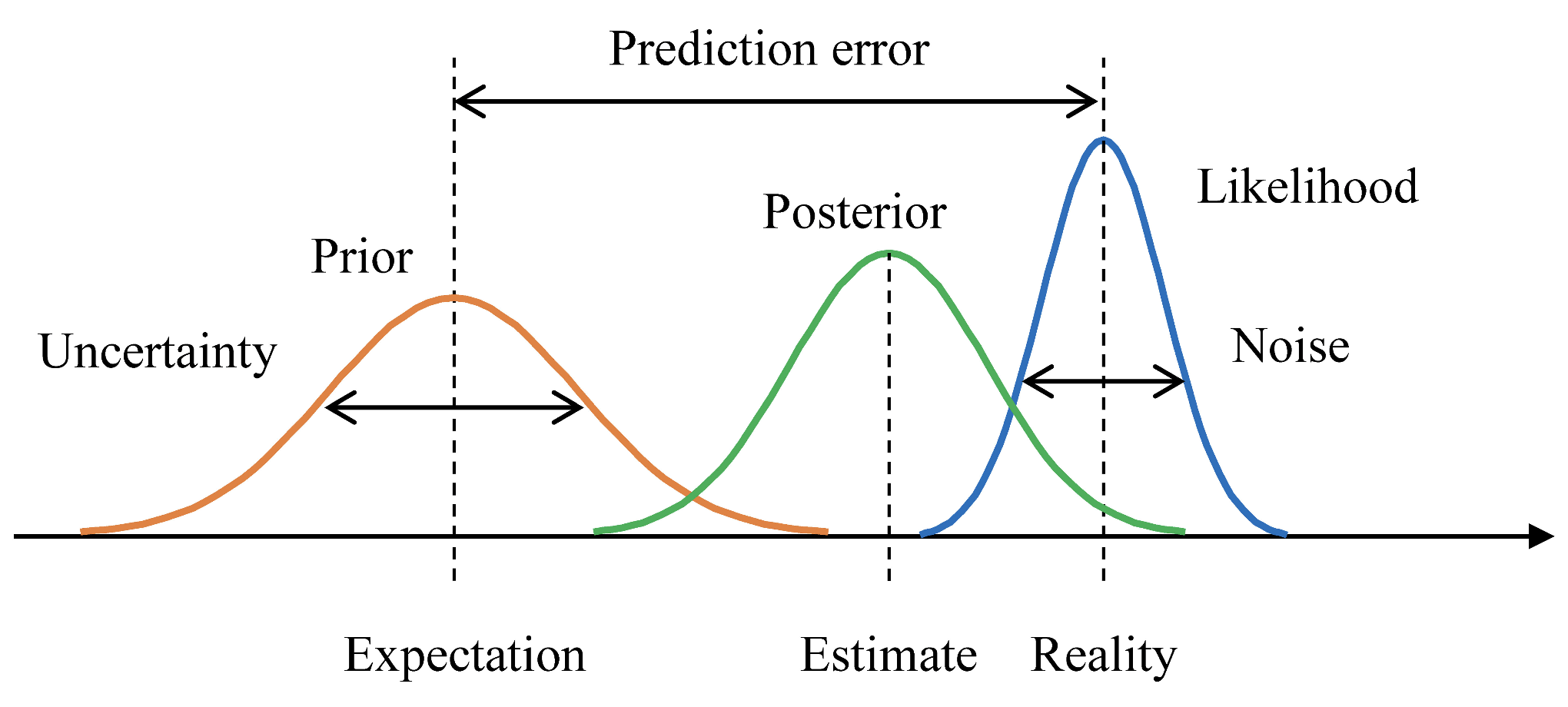
../_images/likelihood_prior_posterior.png

Figure 1. Example of Bayesian inference with a prior distribution, a posterior distribution, and a likelihood function. Taken from Yanagisawa, Kawamata, and Ueda (2019).

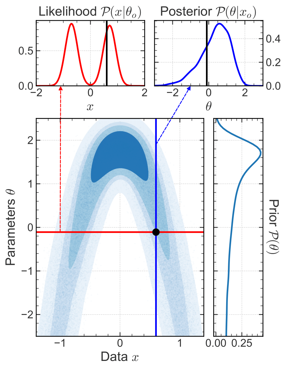
Figure 2. Prior, likelihood and posterior distributions for an arbitrary 1D inference problem. The observed data point $x_0$ and the true parameter $\theta_0$ are indicated in black. In a Bayesian setting, we want to infer the posterior distribution on the model parameter $\theta$ given the data (blue). Conversely, if we know the true parameter $\theta_0$ then we get the likehood (red), i.e. the probability distribution of the data. Taken from Ho et al. (2024).

Let’s remind ourselves of what the Likelihood function is:#

The likelihood function quantifies how likely the observed data is given a set of model parameters that describe our theory. Essentially, the likelihood is what we know about how the data was generated and it describes the underlying probabilistic process the data has to go through based on the model and its parameters.

Given some data/observations $x$, generated through some stochastic process, we can sometimes construct a likelihood function that describes the probability of observing the data given some parameters $\theta$.

Normally, we derive the analytical form of the likelihood function from the theory, combined with some assumptions about the noise in the data or unknown physics (e.g. assume Gaussian distribution for continuous data, Poisson distribution for count data).

The limits of traditional inference:#

What we have described so far is the traditional Bayesian inference, where we write down an analytical form of the likelihood. Afterwards, we can sometimes analytically compute the posterior distribution (if the evidence term is tractable) or use sampling methods (e.g. MCMC) to sample from it.

However, we often encounter complex systems where the underlying processes are not fully understood or are too complicated to model analytically → for a general inference problem, we may not know which likelihood function to choose or whether this choice is valid.

In-class discussion: What happens when we cannot write down an analytical form of the likelihood?
Discuss with your teammate, then report.

[Spoiler] (click here to expand)

We can resort to…

Simulators#

Simulators are computer programs that generate synthetic data from a model. They take as input a set of parameters $\theta$, sample a series of internal states or latent variables, $z_i \sim p(z_i | z_{<i}, \theta)$, where “~” means “sampling from”, and then generate a data vector $x \sim p(x | z, \theta)$.

In astronomy, some examples of simulators are:

N-body simulations: simulate the evolution of a system of particles under the influence of gravity.
Galaxy formation simulations: simulate the formation and evolution of galaxies (N-body, hydrodynamics, magnetic fields, etc).
Stellar population synthesis: simulate the spectral energy distribution of a stellar population.

The latent variables $z$ can be:

physical quantities that are not directly observable (e.g. position of a particle in an N-body simulation). This may include instrumental effects (e.g. seeing, telescope properties).
non-physical quantities that are internal to the simulator, and do not have a direct physical interpretation (e.g. some random seed).

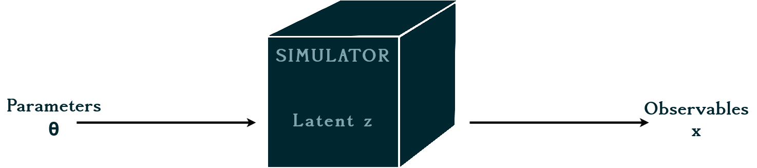
Figure 3. The simulator takes as input the model parameters $\theta$ and generates synthetic data $x$. We can view the simulator as a black box function that can be used to generate data for any set of parameters..

The question is:

How can we use simulations to perform inference?

Simulation-based inference: The basic idea#

Instead of trying to analytically evaluate the likelihood, we can build a forward model of the data → the stochastic simulator becomes the physical model.

The outputs of the simulator become in this way samples of the observational data that we would expect to observe given the parameters $\theta$. So, running the simulator at a fixed $\theta$ draws a sample $x \sim p(x \mid \theta)$.

Therefore, if we simulate enough examples, their relative frequency traces out the full distribution $p(x \mid \theta)$. That is, we can characterize the likelihood directly from simulations, without ever writing it down analytically!

This way, we can:

bypass the need to evaluate the likelihood analytically
fully exploit the information content of the data
incorporate complex physical models, and systematic effects
combine multiple probes via joint simulations

So why hasn’t this been mainstream until now?

The challenge of simulation-based inference#

The probability of a simulation run depends jointly on the observation and the stochastic latent variables $z$ of the simulator: $p(x,z | \theta)$.

However, we only observe the data $x$, so the likelihood we need should be marginalized over the latent variables:

\[ \Large p(x | \theta) = \int p(x,z | \theta) dz = \int p(x | z, \theta) p(z | \theta) dz\]

This is an integral over all possible trajectories through the latent space (i.e. all possible execution traces of the simulator). For realistic simulators, with large latent spaces, it is not feasible to evaluate this integral explicitly.

⮕ the marginal likelihood is intractable!

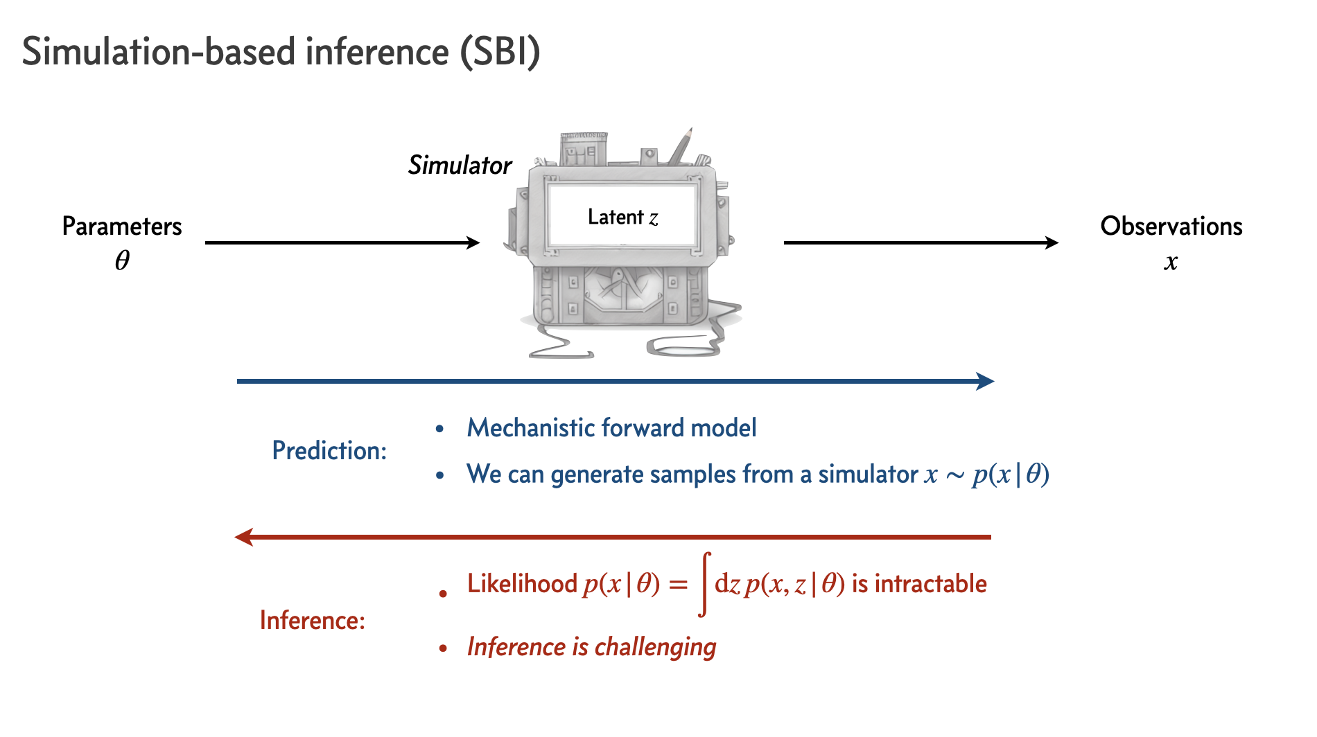
Figure 4. The simulation-based inference (SBI) framework. The simulator is used to generate synthetic data $x \sim p(x | \theta)$ for a range of parameters $\theta$. However, doing inference in this setting is challenging because the likelihood function is intractable. Image credit: Siddharth Mishra-Sharma.

So, how do we deal with this?

A variety of algorithms:

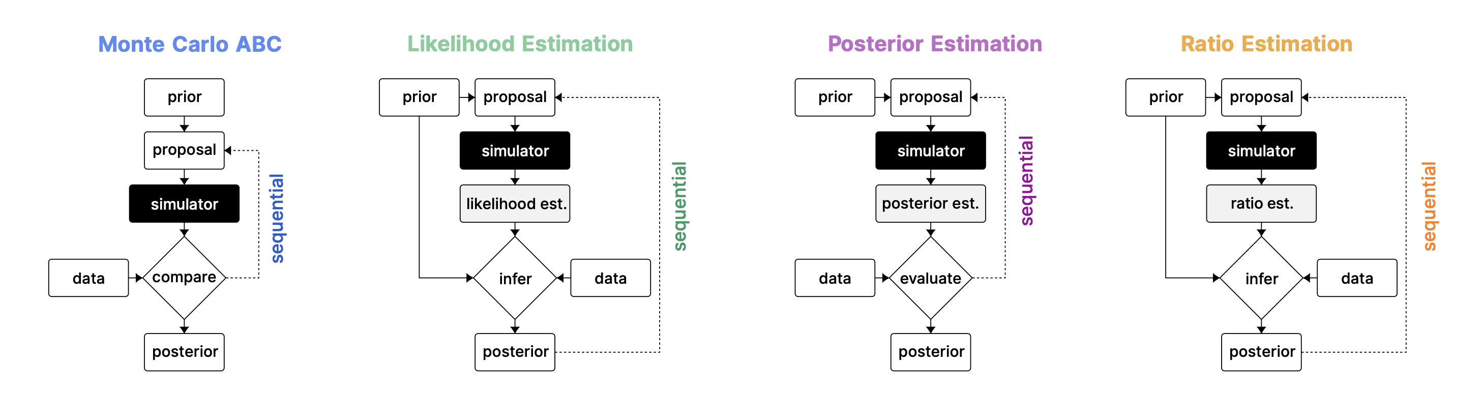
Figure 5. Different simulation-based inference methods. Taken from Lueckmann et al. (2021).

In this version of the lecture, we will cover the first (Approximate Bayesian Computation) and the third (Neural Posterior Estimation) methods. For the other two methods, you can refer to the extended versions of the notebook from previous schools.

Working Example: Cosmology with Supernovae#

We’ll consider a simplified model for the luminosity distance to supernovae, which depends on the cosmological parameters $\Omega_m$ (matter density parameter) and $H_0$ (Hubble constant).

Key concepts:

Luminosity: the total energy output of a supernova in the form of light. Linked to the absolute magnitude.
Apparent magnitude $m$: how bright the supernova appears to us.
Luminosity distance $d_L$: a measure of how far away an object is, based on how faint its light appears compared to its luminosity.

We observe a set of supernovae with apparent magnitudes $m_{\text{obs}}$ at known redshifts $z$. Our model links them to cosmology in two steps. The theoretical apparent magnitude $m_{\text{th}}$ follows from the luminosity distance $d_L$:

\[ \Large m_{\text{th}} = 5 \log_{10}(d_L) + 19.3, \tag{1}\]

where the absolute magnitude for a type Ia supernova is -19.3 (in the V band). For a flat universe ($\Omega_k = 0$), $d_L$ is set by the cosmological parameters $\Omega_m$ and $H_0$ at redshift $z$:

\[ \Large d_L (z) = \frac{c(1+z)}{H_0} \int_0^z \frac{dz'}{\sqrt{\Omega_m(1+z')^3 + (1-\Omega_m)}}, \tag{2}\]

where $c$ is the speed of light.

The problem we will solve is to infer the cosmological parameters $\Omega_m$ and $H_0$ from the observed apparent magnitudes $m_{\text{obs}}$ and redshifts $z$.

Standard Bayesian Inference#

Let’s first try to solve this problem using standard Bayesian inference. We’ll assume that the observed apparent magnitudes $m_{\text{obs}}$ have Gaussian errors, and therefore, we can write down the likelihood function as a Gaussian over the observed data given the parameters $\Omega_m$ and $H_0$:

\[ \Large \mathcal{L}(\Omega_m, H_0) = \prod_{i=1}^N \frac{1}{\sqrt{2\pi\sigma_i^2}} \exp\left[-\frac{(m_{\text{obs},i} - m_{\text{th},i})^2}{2\sigma_i^2}\right], \tag{3}\]

where $N$ is the number of supernovae, $m_{\text{obs},i}$ is the observed apparent magnitude of the $i$-th supernova, $\sigma_i$ is the error in this measurement, and $m_{\text{th},i}$ is the corresponding theoretical apparent magnitude.

First, let’s create some mock observed data to work with. We’ll assume that the redshifts $z$ of the supernovae are known and generate the observed apparent magnitudes $m_{\text{obs}}$ by adding random (Gaussian) noise to the theoretical apparent magnitudes $m_{\text{th}}$:

\[ \Large m_{\text{obs}} = m_{\text{th}} + \mathcal{N}(0, \sigma^2)\]

where $$ \Large \left\{z, H_0, \Omega_m \right\} \xrightarrow{(2)} d_L \xrightarrow{(1)} m_{\text{th}} \; .$$

The following function calculates the luminosity distance given the redshift and cosmological parameters:

# Luminosity distance function
def luminosity_distance(z, Omega_m, H0):
    """ Calculate the luminosity distance for a given redshift, Omega_m and H0 """
    integrand = lambda z_prime: 1.0 / np.sqrt(Omega_m * (1 + z_prime)**3 + (1 - Omega_m))
    d_L = np.array([quad(integrand, 0, z_i)[0] for z_i in z])
    return (c * (1 + z) * d_L) / H0

#random seed
np.random.seed(1234)
torch.manual_seed(1234)

# Constants
c = 299792.458  # Speed of light in km/s

# True cosmological parameters
true_Omega_m = 0.3
true_H0 = 70.0  # Hubble constant in km/s/Mpc

# Redshifts of the supernovae
z = np.linspace(0.01, 1.0, 50)

# Noise level in the observed magnitudes
sigma = 0.5

# Generate synthetic data
d_L_true = luminosity_distance(z, true_Omega_m, true_H0)
m_true = 5 * np.log10(d_L_true) + 19.3  # Apparent magnitude formula
m_obs = m_true + np.random.normal(0, sigma, len(m_true))  # Adding Gaussian noise

# Plot synthetic data
plt.errorbar(z, m_obs, yerr=0.5, fmt='.', label='Observed magnitudes')
plt.plot(z, m_true, label='True magnitudes')
plt.xlabel('Redshift $z$')
plt.ylabel('Apparent magnitude $m$')
plt.legend()
plt.show()

Next, we will adopt a uniform prior for $ 0 < \Omega_m < 1$ and $50 < H_0 < 100$, define the likelihood function from Eq. $(3)$, and the posterior from the Bayes theorem.

# Log-prior function
def log_prior(params):
    Omega_m, H0 = params
    if 0 < Omega_m < 1 and 50 < H0 < 100:
        return 0
    else:
        return -np.inf
    
# Define the log-likelihood function
def log_like(params, z, m_obs):
    Omega_m, H0 = params
    d_L = luminosity_distance(z, Omega_m, H0)
    m_th = 5 * np.log10(d_L) + 19.3  # Theoretical magnitudes
    sigma_m = 0.5  # Assumed standard deviation of magnitudes
    return -0.5 * np.sum(((m_obs - m_th) / sigma_m)**2)    

# Log-posterior function
def log_post(params, z, m_obs):
    lp = log_prior(params)
    if not np.isfinite(lp):
        return -np.inf
    else:
        return lp + log_like(params, z, m_obs)

Now, we just need to sample from the posterior using MCMC to get the distribution of the parameters $\Omega_m$ and $H_0$.

# Sampling with `emcee` 
ndim, nwalkers = 2, 16
ncpus = multiprocessing.cpu_count()

# Initialize walkers around a random position withing the prior volume
pos = np.random.uniform([0, 50], [1, 100], (nwalkers, ndim))

with Pool(ncpus) as pool:
    sampler = emcee.EnsembleSampler(nwalkers, ndim, log_post, args=(z, m_obs), pool=pool)
    sampler.run_mcmc(pos, 3000, progress=True)

# Get samples and convert to GetDist MCSamples
flat_samples = sampler.get_chain(discard=1000, flat=True)

# GetDist plotting
standard_samples = MCSamples(samples=flat_samples, names=['\Omega_m', 'H_0'], labels=['\Omega_m', 'H_0'])

g = plots.get_subplot_plotter(width_inch=6)
g.triangle_plot([standard_samples], filled=True, markers={'\Omega_m': true_Omega_m, 'H_0': true_H0})
plt.show()

Simulation-based Inference#

Now, let’s try to solve the same problem using simulation-based inference methods. To do this, we will first need to construct a simulator for the luminosity distance to supernovae.

# noise level
sigma = 0.5

# Forward model to simulate observed magnitudes
def luminosity_distance_simulator(params, z):
    Omega_m, H0 = params
    d_L = luminosity_distance(z, Omega_m, H0)
    m_th = 5 * np.log10(d_L) + 19.3  # Theoretical magnitudes
    m_sim = m_th + np.random.normal(0, sigma, len(m_th))
    return m_sim

This very simple simulator uses the theoretical models for the apparent magnitude and luminosity distance, for fixed cosmological parameters $\Omega_m$ and $H_0$, given by Eqs. $(1)$ and $(2)$, and adds Gaussian noise to generate the observed apparent magnitudes $m_{\text{obs}}$.

Traditional SBI - Approximate Bayesian Computation (ABC)#

ABC was one of the first simulation-based inference methods developed and is centered on the idea of approximating the posterior distribution by sampling from the prior distribution and accepting samples that are “close enough” to the observed data.

General procedure:

Sample parameters from the prior distribution $\theta \sim p(\theta)$.
Forward simulate using these parameters to generate synthetic observations $x \sim p(x | \theta)$.
Compare the synthetic observations to the real observed data $x_{\text{obs}}$ using a distance metric $d(x, x_{\text{obs}})$.
If the synthetic observations are “close enough” to the real observed data, i.e., $d(x, x_{\text{obs}}) < \epsilon$, for some threshold $\epsilon$, then accept the parameters $\theta$ as samples from the posterior $p(\theta | x_{\text{obs}})$.

ABC does not require the likelihood function to be known, instead the likelihood is approximated by the probability that the condition $d(x, x_{\text{obs}}) < \epsilon$ is satisfied.

As the threshold $\epsilon \to 0$, the accepted samples converge to the true posterior. For $\epsilon > 0$, the inferred posterior will be broader than the true posterior, therefore the inference will result in a conservative estimate.

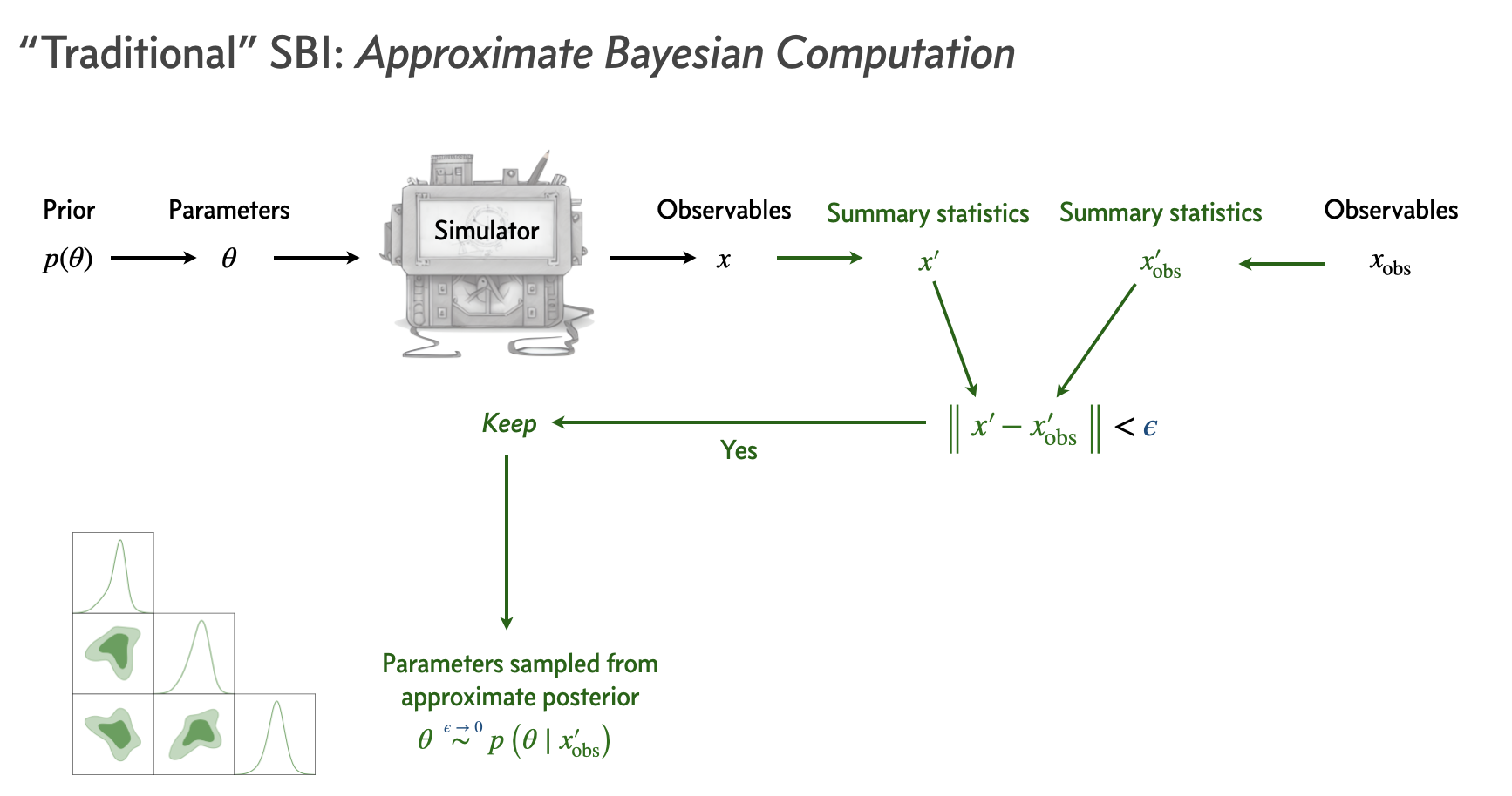
Figure 6: Approximate Bayesian computation (ABC) algorithm. The simulator is used to generate synthetic data $x \sim p(x | \theta)$ for a range of parameters $\theta$. The distance function $d(x, x_{\text{obs}})$ is used to compare the synthetic data to the observed data. Image credit: Siddharth Mishra-Sharma.

Let’s now try to apply ABC to our problem of inferring the cosmological parameters $\Omega_m$ and $H_0$ from supernova data. As a distance metric, we’ll use the mean squared error (MSE):

\[ \Large d(x, x_{\text{obs}}) = \frac{1}{N} \sum_{i=1}^N (x_i - x_{\text{obs},i})^2 \]

between the observed apparent magnitudes $m_{\text{obs}}$ and the synthetic apparent magnitudes $m_{\text{th}}$.

# Distance metric: Mean Squared Error
def mse(x, x_sim):
    return np.sum((x - x_sim) ** 2) / len(x)

# ABC Algorithm
def abc(y, x, eps_thresh=0.5, num_samples=1000):
    """ Approximate Bayesian Computation (ABC) algorithm """
    accepted_samples = []
    trials = 0
    progress_bar = tqdm(total=num_samples, desc=f"Accepted Samples (eps={eps_thresh})")

    while len(accepted_samples) < num_samples:
        params = np.random.uniform(low=[0, 50], high=[1, 100])  # θ ~ p(θ) (Step 1)
        x_sim = luminosity_distance_simulator(params, y)  # x ~ p(x|θ) (Step 2)
        eps = mse(x, x_sim)  # Distance metric; d(x, x_sim) (Step 3)
        trials += 1

        # If accepted, add to samples (Step 4)
        if eps < eps_thresh:
            accepted_samples.append(params) 
            acceptance_ratio = len(accepted_samples) / trials 
            progress_bar.update(1)
            progress_bar.set_postfix(acceptance_ratio=f"{acceptance_ratio:.3f}")

    progress_bar.close()
    
    return np.array(accepted_samples)

We will run the ABC algorithm for two different values of $\epsilon$: $0.4$ and $0.6$.

# Run ABC
eps_thresh = [0.4, 0.6]

# Run ABC for each epsilon threshold
results = {}
for eps in eps_thresh:
    results[eps] = abc(z, m_obs, eps_thresh=eps, num_samples=1000)

# GetDist plotting
samples1 = MCSamples(samples=results[0.6], names=['Omega_m', 'H0'], labels=[r'\Omega_m', 'H_0'])
samples2 = MCSamples(samples=results[0.4], names=['Omega_m', 'H0'], labels=[r'\Omega_m', 'H_0'])

g = plots.get_subplot_plotter(width_inch=6)
g.triangle_plot([samples1, samples2], filled=True, markers={'Omega_m': true_Omega_m, 'H0': true_H0}, legend_labels=[ f"eps={eps_thresh[1]}", f"eps={eps_thresh[0]}"] )
plt.show()

In-class discussion: What can you see from running the ABC algorithm and the plot?
Discuss with your teammate, then report.

[Spoiler] (click here to expand)

We see that first of all, the posteriors that we get from ABC are reasonably close to the “true” posterior that we got from standard Bayesian inference. However, as expected, the posteriors from ABC are broader than the true posterior, because of the relatively large values of ε that we used, and indeed, the bigger the ε, the broader the posterior.

In-class discussion: What do you think are the main drawbacks of ABC?
Discuss with your teammate, then report.

[Spoiler] (click here to expand)

We need to choose a distance metric that is appropriate for the problem.
We have an extra hyperparameter to tune: the threshold ε.
Small values of ε require unfeasibly many simulations, while large values lead to reduced accuracy.
The sample efficiency of ABC scales poorly to high-dimensional data x and high-dimensional parameters θ.
Inference for new data or different choice of prior requires re-running the entire algorithm.

Neural Posterior Estimation (NPE)#

This method is a Deep Learning implementation of density estimation: given a set of points $\{u\} \sim \mathcal{P}(u)$, we want to learn the distribution $\mathcal{P}(u)$.

The way that we would normally do this for inference is by creating a model for the likelihood via estimating the distribution of the simulated data using histograms or kernel density estimation. However, these methods are not very flexible and do not scale well to high-dimensional data (curse of dimensionality).

This is where recent advances in density estimation techniques using neural networks come in.

To understand how neural networks can be used for density estimation, let’s first consider a simple example where we want to estimate the distribution over $\theta$, in the case when this distribution is a 1D Gaussian. Here, we can use a neural network to model the mean and variance of the Gaussian as a function of some input $x$:

\[ \Large p(\theta | x) = \mathcal{N}\big(\mu = f(x), \sigma = g(x)\big),\]

where $f(x)$ and $g(x)$ are the outputs of the neural network. The neural network will be trained to fit the training data by tuning the parameters of $f$ and $g$.

However, in general, we do not expect the posterior to be Gaussian. In this case, we can use a more general neural network architecture to model the posterior. One class of these neural density estimation methods is Normalizing Flows.

Interlude: Normalizing Flows#

Normalizing Flows are a class of generative models — the same family behind the AI image generators you may have heard so much about (DALL·E, Stable Diffusion, Midjourney). A generative model learns a probability distribution from data and can then draw new samples from it: an image generator trained on millions of pictures effectively learns the distribution of natural images, and “generating an image” is just sampling from that distribution.

A Normalizing Flow does this through invertible transformations of the probability space that map a simple distribution to a more complex one.

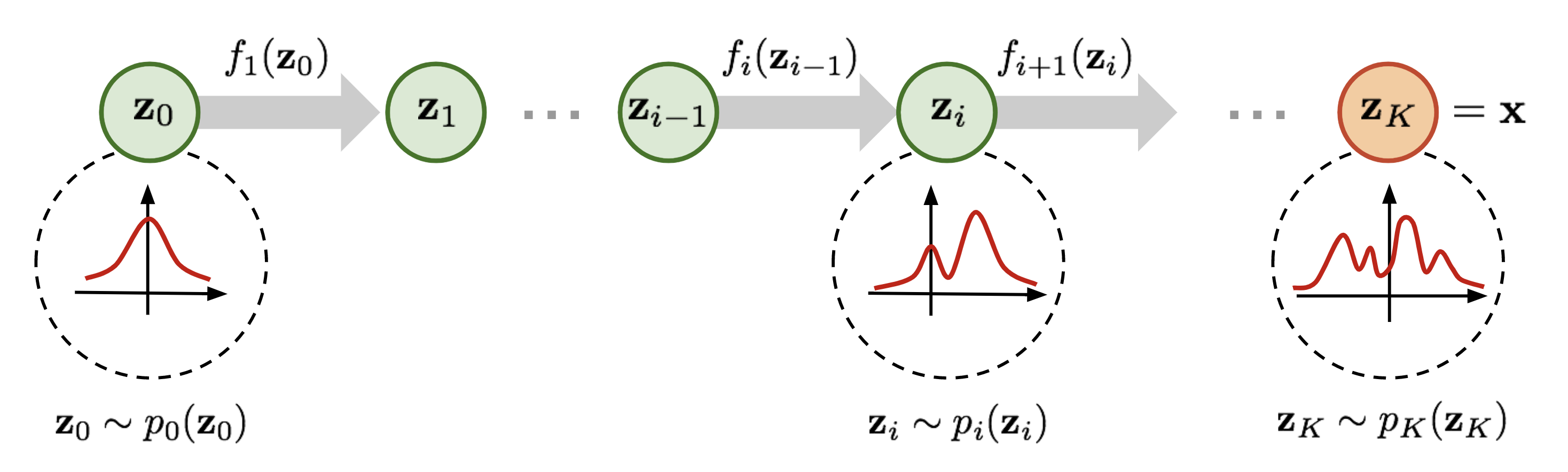
Figure 7: Illustration of a Normalizing Flow model, transforming a simple distribution $p_0(z_0)$ (left) to a complex one $p_K(z_K)$ (right) through a series of invertible transformations $f_k$. Image credit: Lilian Weng.

The key idea behind Normalizing Flows is to start with a simple base distribution $\pi(\mathbf{u})$ (e.g. a standard normal) and transform it through a series of invertible transformations $f$ (bijections) to obtain a more complex target distribution $p(\mathbf{x})$. This is formalized using the change of variables formula:

\[ \Large \mathbf{u} \sim \pi(\mathbf{u}), \quad \mathbf{x} = f(\mathbf{u}), \quad \mathbf{u} = f^{-1}(\mathbf{x}) \]

\[ \Large p(\mathbf{x}) = \pi(\mathbf{u}) \left| \det \frac{d\mathbf{u}}{d\mathbf{x}} \right| = \pi(f^{-1}(\mathbf{x})) \left| \det \frac{df^{-1}(\mathbf{x})}{d\mathbf{x}} \right|\]

where $f^{-1}$ is the inverse transformation of $f$, and the Jacobian determinant $\left| \det \frac{df^{-1}(\mathbf{x})}{d\mathbf{x}} \right|$ accounts for the change in probability volume corresponding to and element $\mathrm{d} \mathbf{u}$ when transforming from $\mathbf{u}$ to $\mathbf{x}$ space. This factor compensates for how $f$ transforms, stretches, or compresses volume locally, so that the resulting density $p(\mathbf{x})$ remains correctly normalized (integrates to 1). Normalizing Flows allow constructing expressive distributions by composing simple, invertible transformations.

The challenge is in designing mappings $f$ that are both: easy to invert and easy to compute the Jacobian of.

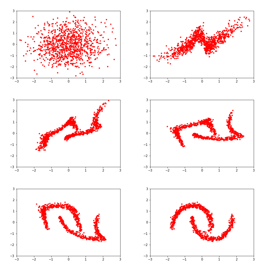
Figure 8: The Normalizing Flow transforms the simple base distribution to the target distribution by applying a series of invertible transformations one after the other. Axes are in arbitrary units. Image credit: Eric Jang.

Training a Normalizing Flow (Open at your own risk)

Training#

Normalizing Flows are trained to maximize the likelihood of training data $x$ under the transformed distribution $p(x)$. This is equivalent to minimizing the Kullback-Leibler divergence between the data and model distributions.

Kullback-Leibler (KL) divergence measures the difference between two probability distributions $p(x)$ and $q(x)$:

\[ D_{KL}(p||q) = \mathbb{E}_{p(x)}\left[\log \frac{p(x)}{q(x)}\right] = \int p(x) \log \frac{p(x)}{q(x)} dx.\]

The KL divergence is non-negative and is zero if and only if $p(x) = q(x)$. Minimizing the KL divergence is equivalent to maximizing the likelihood of the data under the model distribution.

Let’s see how we would train a Normalizing Flow to estimate the posterior $p(\theta | x)$. So far, we have the tools to emulate a probability distribution with a neural network. We’ll write such a probability distribution $q_\phi$ where $\phi$ are the parameters of the neural network.

A way to learn the distribution $p(\theta | x)$ by a Neural Network with weights $\phi$ is to minimize $D_{KL}\Big(p(\theta | x) || q_\phi(\theta | x)\Big)$ with respect to the network parameters $\phi$. Let’s do the math:

\[ D_{KL}\Big(p(\theta | x) || q_\phi(\theta | x)\Big) = \mathbb{E}_{p(\theta | x)}\left[\log \frac{p(\theta | x)}{q_\phi(\theta | x)}\right] \]

However, we want our model to work for different values of $x$, so we need to take the expectation of this expression with respect to $p(x)$:

\[\begin{align*} \mathbb{E}_{p(x)} \Big[ D_{KL}\big(p(\theta | x) || q_\phi(\theta | x)\big) \Big] &= \mathbb{E}_{p(x)}\mathbb{E}_{p(\theta | x)}\left[\log \frac{p(\theta | x)}{q_\phi(\theta | x)}\right] = \mathbb{E}_{p(\theta,x)}\left[\log \frac{p(\theta | x)}{q_\phi(\theta | x)}\right] \\\\ &= \mathbb{E}_{p(\theta,x)} \left[ - \log q_\phi(\theta | x)\right] + \mathrm{const}_{w.r.t. \phi} \end{align*}\]

where in the second equality we used $p(\theta,x) = p(\theta | x)p(x)$. Therefore, to optimize our neural network, we need to minimize:

\[ \min_\phi \mathbb{E}_{p(x)} \Big[ D_{KL}\big(p(\theta | x) || q_\phi(\theta | x)\big) \Big] = \min_\phi \mathbb{E}_{p(\theta,x)} \left[ - \log q_\phi(\theta | x)\right] + \cancel{\mathrm{const}_{w.r.t. \phi}} \]

which we can estimate because we have samples of $p(\theta,x)$ from the simulator!

Once we have trained the Normalizing Flow, we can sample the model $q_\phi(\theta | x_{\text{obs}})$ directly to obtain samples from the approximate posterior distribution $p(\theta | x_{\text{obs}})$. To do this, we simply sample $z$ from the base distribution (e.g. a standard normal) and apply the inverse transformation $f^{-1}$ to obtain samples from the posterior.

Normalizing Flows summary:#

Start from a simple base distribution that is easy to sample from and evaluate the Jacobian of, like a standard normal.
Apply a sequence of invertible transformations to this base distribution. Each transformation is designed to be efficient to compute and have a tractable Jacobian.
The transformed distribution at the end of this sequence of transformations is the final Normalizing Flow distribution. It can be much more complex and expressive than the base distribution.
Sampling from the Normalizing Flow is efficient - just sample from the base distribution and pass it through the sequence of transformations. Evaluating the density of a volume element is also tractable using the change of variables formula.
The transformations are parameterized by neural networks and trained to maximize the likelihood of observed data. This allows learning complex, data-driven distributions.

If you want to learn more about Normalizing Flows, you can check out the paper by Papamakarios et al. (2019) and the blog post by Lilian Weng.

Back to NPE#

Now that we are OK with Normalizing Flows, let’s see the specifics of how we can use them for Neural Posterior Estimation. The steps of the algorithm are:

Generating the training data: Sample a large number of parameter values $\theta$ from the prior, run the simulator to generate corresponding data $x$, and store the $(\theta, x)$ pairs as training data.
Training the conditional density estimator:
- evaluate the log-density of the Normalizing Flow, $\log q_\phi(\theta | x)$, at the training data points $(\theta, x)$.
- train for the parameters $\phi$ of the Normalizing Flow until the log-likelihood of the training data is maximized.
- the exact loss function is: $$ \Large \mathcal{L}(\phi) = -\frac{1}{N} \sum_{i=1}^N \log q_\phi(\theta_i | x_i),$$ where $N$ is the number of training samples, and $\phi$ are the parameters of the Normalizing Flow.
Inference: To perform inference for new data $x_{\text{obs}}$, just sample from the model $q_\phi(\theta | x_{\text{obs}})$ to obtain samples from the posterior distribution $p(\theta | x_{\text{obs}})$!

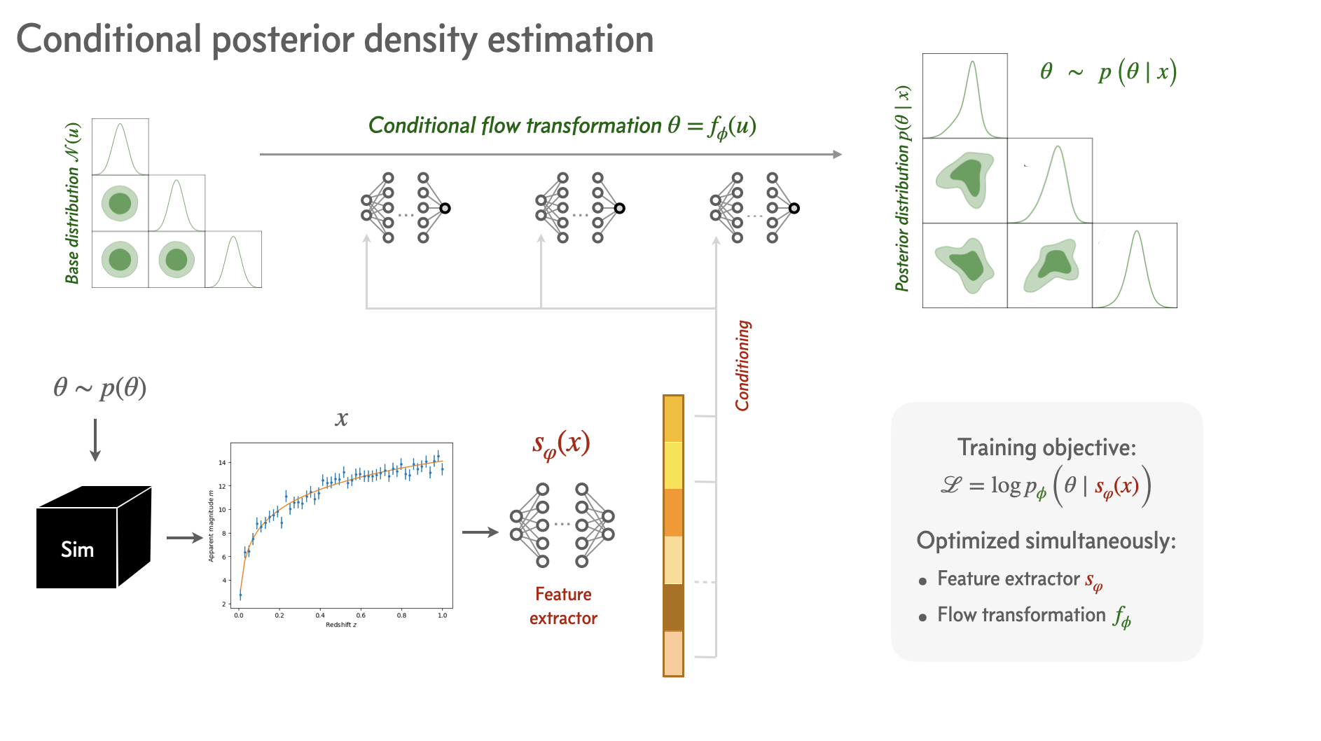
Figure 9: Neural Posterior Estimation (NPE) algorithm. The simulator is used to generate synthetic data $x$ for a range of parameters $\theta$. The Normalizing Flow is trained to model the posterior distribution $p(\theta | x)$ conditioned on the training data. Image credit: Siddharth Mishra-Sharma.

Applying NPE to our problem#

To use SBI methods like NPE, we can leverage existing libraries that implement these algorithms. Those can make your life much easier, and you can use them to perform SBI without having to make everything from scratch. Some of the most popular libraries are:

Let’s see how easy things can be using e.g. the sbi library. We just need to take our simulated pairs of $(\theta, x)$ and choose an SBI method. So let’s do it with NPE:

Sample generation#

This method is based on Neural Networks, and to train them, we need to generate a large number of samples from the simulator. So let’s sample from the prior distribution of the parameters $\theta$ and then simulate the data $x$ for each of these parameters:

np.random.seed(1234) # use random seed for reproducibility

# Generate training data
n_train = 20_000
param_samples = np.random.uniform(low=[0, 50], high=[1, 100], size=(n_train, 2)) # Parameter proposal
x_samples = np.array([luminosity_distance_simulator(theta, z) for theta in tqdm(param_samples)])

# Convert from numpy arrays to pytorch tensors
param_samples = torch.tensor(param_samples, dtype=torch.float32)
x_samples = torch.tensor(x_samples, dtype=torch.float32)

Check one of the generated samples:

# plot the training data
plt.errorbar(z, x_samples[42], yerr=sigma, fmt='.', label='Simulated data')
plt.xlabel('Redshift $z$')
plt.ylabel('Apparent magnitude $m$')
plt.legend()
plt.show()

NPE class#

Now the important part: we will define our SBI model that will learn the posterior distribution $p(\theta | x)$.

It will be trying to model the distribution of the parameters $\theta$ given the data $x$.

prior = BoxUniform(low=torch.tensor([0.0, 50.0]), high=torch.tensor([1.0, 100.0]))

# Define the SBI model and give it the prior
inference = SNPE(prior=prior)

# append the parameter-simulation pairs
inference.append_simulations(param_samples, x_samples)

# train() the density estimator
density_estimator = inference.train()

# build posterior using the trained density estimator
posterior = inference.build_posterior(density_estimator)

⚠️ NOTE: in the newer versions of sbi, the API has changed a bit. So the cell above would look like this:

import sbi
from sbi.inference import NPE

inference = NPE()
inference.append_simulations(param_samples, x_samples).train()
posterior = inference.build_posterior()

We have trained the Normalizing Flow model to estimate the posterior distribution $p(\theta | x)$ given any observed data $x$! We can now sample from this model to obtain samples from the posterior distribution for $\Omega_m$ and $H_0$.

Inference#

Let’s generate a mock set of observed data $x_{test} = x_{\text{obs}}$ and obtain samples of the posterior distribution $p(\theta | x_{\text{obs}})$ from the trained model. Don’t get confused - in a real application, $x_{\text{obs}}$ would be the actual observed data, and we would use the model to infer the posterior distribution of the parameters $\theta$ given this data.

# Obtain a mock observation from the trained model
param_test = np.array([0.3, 70.0])
x_obs = luminosity_distance_simulator(param_test, z) # assume that the observed data "comes from" the above parameters

Nice, now we can just sample from the posterior distribution using the trained model, conditioned on the observed data $x_{\text{obs}}$, and make the corner plot of the posteriors:

samples_npe = posterior.sample((10000,), x=x_obs)

# Convert to numpy (ensure on CPU and detached from graph)
if isinstance(samples_npe, torch.Tensor):
    samples_npe = samples_npe.detach().cpu().numpy()
else:
    samples_npe = np.asarray(samples_npe)


# Create a getdist MCSamples object
samples  = MCSamples(samples=flat_samples, names=['Omega_m', 'H0'], labels=[r'\Omega_m', 'H_0'])
gd_samples_npe = MCSamples(samples=samples_npe, labels=['\Omega_m', 'H_0'], names=['\Omega_m', 'H_0'])

# Make a triangle/contour plot with getdist
g = plots.get_subplot_plotter(width_inch=6)
g.triangle_plot([gd_samples_npe], filled=True, markers={'\Omega_m': true_Omega_m, 'H_0': true_H0}, legend_labels=['NPE'])

We see that the posteriors that we get from NPE are very similar to the “true” posterior that we got from standard Bayesian inference!

But be careful, sometimes things can go wrong , so you may have to look in the details of the code of the library, change stuff, and all those horrible things that you don’t want to do. But now you know how everything works under the hood, so you can do it!

What if we wanted to make everything from scratch? (optional / bonus)#

Let’s see what happens behind the scenes…

np.random.seed(1234) # use random seed for reproducibility

# Generate training data
n_train = 50_000
param_samples = np.random.uniform(low=[0, 50], high=[1, 100], size=(n_train, 2)) # Parameter proposal
x_samples = np.array([luminosity_distance_simulator(theta, z) for theta in tqdm(param_samples)])

# Convert to tensors
param_samples = torch.tensor(param_samples, dtype=torch.float32)
x_samples = torch.tensor(x_samples, dtype=torch.float32)

We will try to implement NPE from scratch using PyTorch and a Normalizing Flow model.

For the training data, we will use the same samples that we generated before: pairs of $(\theta, x)$.

In machine learning, it is common to normalize the input data to have zero mean and unit variance (this is done automatically in the sbi package). This helps the neural network to learn more efficiently:

def normalize(data):
    """ Normalizes the data to have mean 0 and standard deviation 1. """
    mean = data.mean(dim=0)
    std = data.std(dim=0)
    return (data - mean) / std, mean, std

# Normalize the training data
x_norm, x_mean, x_std = normalize(x_samples)
param_norm, param_mean, param_std = normalize(param_samples)

Featurizer#

We will define a simple Mutli-Layer Perceptron, which will reduce the dimensionality of the data $x$ and serve as the feature extractor $s_\phi(x)$ in the NPE algorithm (see Fig. 9). Don’t worry too much about this for now, just consider $s_\phi(x) = x$.

def build_mlp(input_dim, hidden_dim, output_dim, num_layers, activation=nn.GELU()):
    """Builds a multi-layer perceptron (MLP) neural network."""
    layers = [nn.Linear(input_dim, hidden_dim), activation]  # First layer and activation
    
    for _ in range(num_layers):
        layers += [nn.Linear(hidden_dim, hidden_dim), activation] # Hidden layers and activations
        
    layers += [nn.Linear(hidden_dim, output_dim)] # Output layer
    
    return nn.Sequential(*layers)

NPE class#

Now the important part: we will define our conditional Normalizing Flow model that will learn the posterior distribution $p(\theta | x)$.

The Normalizing Flow will be trying to model the distribution of the parameters $\theta$ given the context (condition) of the data $x$.

class NeuralPosteriorEstimator(pl.LightningModule):
    """
    Neural Posterior Estimator using a normalizing flow as the posterior density estimator.

    Parameters:
        featurizer (nn.Module): Neural network for feature extraction.
        d_context (int): Dimension of the context vector.
    """
    
    def __init__(self, featurizer, d_context=16):
        super().__init__()
        self.featurizer = featurizer # Featurizer network for context extraction
        self.flow = self._build_flow(d_in=2, d_hidden=32, d_context=d_context, n_layers=4) # Normalizing flow
    
    def _build_flow(self, d_in, d_hidden, d_context, n_layers):
        """ Instantiate a normalizing flow with Masked Autoregressive Transformations. """
        base_dist = StandardNormal(shape=[d_in]) # base distribution of NF = standard normal 
        transforms = [] # List to hold the series of transformations
        
        for _ in range(n_layers):
            # Reverse permutation to shuffle the features
            transforms.append(ReversePermutation(features=d_in))
            
            # Masked Autoregressive Transform for flexible and expressive transformations
            transforms.append(MaskedAffineAutoregressiveTransform(features=d_in, hidden_features=d_hidden, context_features=d_context))
            
        # Combine all transformations into a composite transform
        transform = CompositeTransform(transforms)
        
        return Flow(transform, base_dist)    

    def forward(self, x):
        return self.featurizer(x) # Extract features using the featurizer
    
    def loss(self, x, params):
        context = self(x)  # Extract context from x using the featurizer
        return -self.flow.log_prob(inputs=params, context=context) # Compute negative log probability

    def training_step(self, batch):
        x, params = batch 
        loss = self.loss(x, params).mean()  # Compute mean loss
        self.log("train_loss", loss) # Log the training loss
        return loss

    def validation_step(self, batch):
        x, params = batch
        loss = self.loss(x, params).mean() # Compute mean validation loss
        self.log("val_loss", loss) # Log the validation loss
        return loss

    def configure_optimizers(self):
        return torch.optim.Adam(self.parameters(), lr=3e-4) 

Instantiate the featurizer and NeuralPosteriorEstimator

featurizer = build_mlp(input_dim=50, hidden_dim=128, output_dim=16, num_layers=4)
npe = NeuralPosteriorEstimator(featurizer=featurizer, d_context=16)

Create the dataset and dataloader, using the PyTorch DataLoader class:

val_fraction = 0.1 # Fraction of data to use for validation
batch_size = 128 
n_samples_val = int(val_fraction * len(x_norm)) 

dataset = TensorDataset(x_norm, param_norm) 
dataset_train, dataset_val = random_split(dataset, [len(x_samples) - n_samples_val, n_samples_val]) 

train_loader = DataLoader(dataset_train, batch_size=batch_size, num_workers=8, pin_memory=True, shuffle=True)
val_loader = DataLoader(dataset_val, batch_size=batch_size, num_workers=8, pin_memory=True, shuffle=False)

Train the model:

trainer = pl.Trainer(max_epochs=20)
trainer.fit(model=npe, train_dataloaders=train_loader, val_dataloaders=val_loader)

We have trained the Normalizing Flow model to estimate the posterior distribution $p(\theta | x)$ given any observed data $x$! We can now sample from this model to obtain samples from the posterior distribution for $\Omega_m$ and $H_0$.

Inference#

So let’s generate a mock observed data $x_{test} = x_{\text{obs}}$ and sample from the model to obtain samples from the posterior distribution $p(\theta | x_{\text{obs}})$. Don’t get confused - in a real application, $x_{\text{obs}}$ would be the actual observed data, and we would use the model to infer the posterior distribution of the parameters $\theta$ given this data.

# Test the trained model
param_test = np.array([0.3, 70.0])
x_obs = luminosity_distance_simulator(param_test, z) # assume that the observed data "comes from" the above parameters

x_obs_norm = (torch.Tensor(x_obs) - x_mean) / x_std # normalize the test data
context = npe.featurizer(x_obs_norm).unsqueeze(0)

# Sample from the trained normalizing flow
test_samples = npe.flow.sample(num_samples=10000, context=context) * param_std + param_mean
test_samples = test_samples.detach().numpy().squeeze(0)

# Create a MCSamples instance
samples = MCSamples(samples=test_samples, labels=['\Omega_m', 'H_0'], names=['Omega_m', 'H_0'])

true_Omega_m = 0.3
true_H0 = 70

# Create a GetDist plot
g = plots.get_subplot_plotter(width_inch=6)
g.triangle_plot([samples], filled=True, markers={'Omega_m': true_Omega_m, 'H_0': true_H0})
plt.show()

Conclusion#

Advantages of NPE:

No need for a likelihood function.
Get direct samples from the posterior.
Flexible posterior modeling with Normalizing Flows.
Scalable to high-dimensional data and parameters: Normalizing Flows allow NPE to scale to high-dimensional parameter and data spaces.
Amortized inference: Once the Normalizing Flow model is trained on simulated data, it can quickly produce posterior samples for any new observed data $x_{obs}$ through a simple forward pass. This means that we don’t need to re-run the inference algorithm for new data.

Drawbacks of NPE:

We must retrain the model if we want to change the prior.
If the prior and the posterior are very different, the model may not be able to capture the posterior distribution well.
Still, in high-dimensional spaces, the model may struggle to capture the posterior distribution accurately if we don’t have a huge amount of training data.

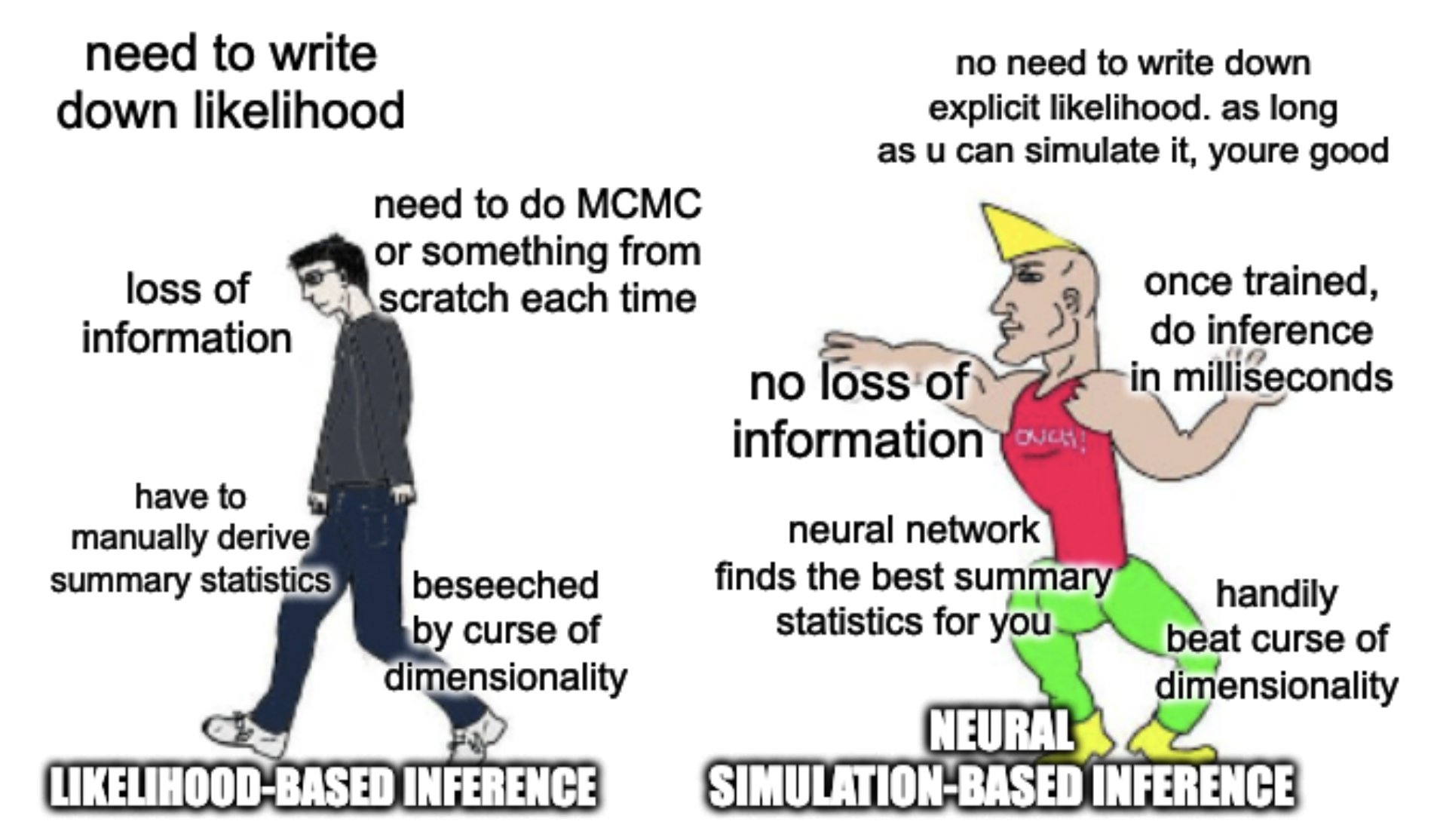
Sources & Further Reading#

This notebook is based on the following sources:

https://github.com/smsharma/sbi-lecture-mit
https://astroautomata.com/blog/simulation-based-inference/
https://github.com/maho3/ltu-ili/tree/main
https://indico.mitp.uni-mainz.de/event/332/contributions/4532/
https://indico.cern.ch/event/768915/contributions/3474655/
https://github.com/glouppe/ssi2023
https://lilianweng.github.io/posts/2018-10-13-flow-models/
https://gebob19.github.io/normalizing-flows/
https://arxiv.org/abs/1911.01429
https://arxiv.org/abs/2402.05137
https://arxiv.org/abs/2101.04653
https://arxiv.org/abs/2403.14750

Suggestions for further reading:

Blogs and general papers:
# EOF

Introduction to Simulation Based Inference

Contents

Introduction to Simulation Based Inference#

Setup#

Introduction#

Revisiting Bayesian Inference#

Let’s remind ourselves of what the Likelihood function is:#

The limits of traditional inference:#

Simulators#

Simulation-based inference: The basic idea#

The challenge of simulation-based inference#

Working Example: Cosmology with Supernovae#

Standard Bayesian Inference#

Simulation-based Inference#

Traditional SBI - Approximate Bayesian Computation (ABC)#

Neural Posterior Estimation (NPE)#

Interlude: Normalizing Flows#

Training#

Normalizing Flows summary:#

Back to NPE#

Applying NPE to our problem#

Sample generation#

NPE class#

Inference#

What if we wanted to make everything from scratch? (optional / bonus)#

Featurizer#

NPE class#

Inference#

Conclusion#

Sources & Further Reading#