
Introduction to Deep Learning#
A quick introductory session on what Deep Learning is and how it has been applied in Astronomy.
Setup#
import numpy as np
import pandas as pd
import matplotlib.pyplot as plt

from IPython.display import display, HTML
display(HTML("<style>.container { width:100% !important; }</style>"))

import requests

url = "https://raw.githubusercontent.com/AstroStat-Academy/assets-public/main/colab/clone_and_cd_colab.py"
colab = requests.get(url).text
exec(colab)

url = "https://raw.githubusercontent.com/AstroStat-Academy/assets-public/main/styles/plot_style.py"
style = requests.get(url).text
exec(style)
Why Deep Learning is cool#
It is not, we are geeks, and that's the truth.
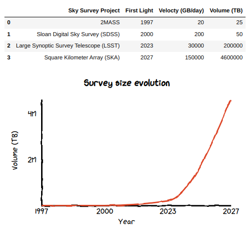
However … we do live in the era of “Big Data”:
|
Figure 1. Current and projected survey size evolution. |
We cannot expect to humanly inspect these data and derive the intuition for the rules which categorize them.
\(\rightarrow\) We have to leverage on:
the large number of examples
algorithms that can abstract arbitrarily complex rules
How does Deep Learning addresses big data issues?#
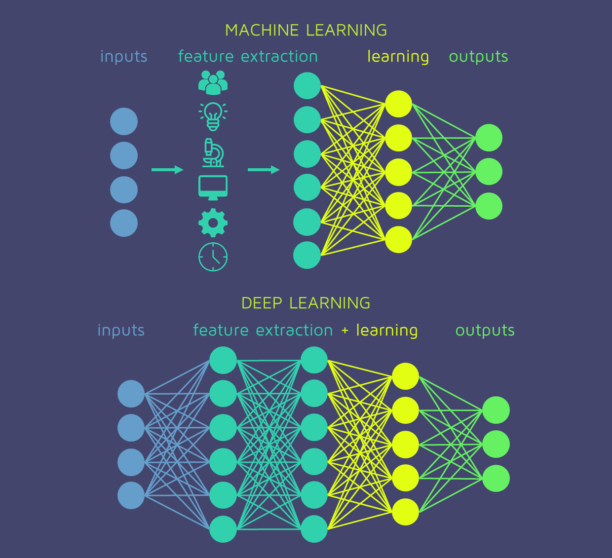
The basic idea is that layers construct new features.
In practice, Deep Learning systems include implicit feature engeneering on top of the learning task (e.g., classificaton or regression).
In this way, they are a step forward with respect to “classic” ML approaches:
|
Figure 2. A Deep Neural Network seen as a combination of feature extractor + learner (e.g. classifier or regressor). (From here) |
From this perspective, the connections between the network neurons represent potential correlations betweeen features.
What are the implications?
The scientist does not have to get detailed insight of the problem to build the proper features or select the proper classifier
\(\rightarrow\) the DL system does it all for us!
This comes particularly handy when we deal with databases with millions of objects and hundreds of features!
References
In case you are curious, it has been proven that Deep Neural Networks are indeed “universal approximators” (e.g. Kurt Hornik, 1991, Neural Networks, 4, 2), meaning that they can in principle explain any linear or non-linear relation beteen the features and the target.
Historical excursus#
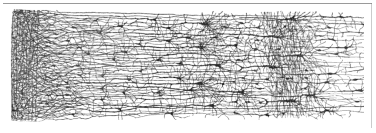
The history of NNs is troubled. Arguably, NNs have been originally inspired by biological neurons.
1943 \(\rightarrow\) Warren McCulloch (neurophysiologist) and Walter Pitts (mathematician)
Simplified computational model of how biological neurons might work together in animal brains
|
Figure 3. Neuron layers in the human cortex. (Adapted from Figure 10-2 of Gerone A. 2017) |
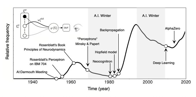
mid’40s\(-\)’60s \(\hspace{0.6cm}\) \(\rightarrow\) Follows some interest and development of early models (e.g. Perceptron)
’70s\(-\)mid’80s \(\hspace{0.6cm}\) \(\rightarrow\) NNs cannot scale efficiently, they get disregarded
mid’80s\(-\)mid’90s \(\rightarrow\) The invention of backpropagation allows to train complex NNs, but …
mid’90s-2010s \(\hspace{0.5cm}\) \(\rightarrow\) Other techniques look simpler, more powerful (e.g. SVM)
2010s\(-\)present \(\hspace{0.3cm}\) \(\rightarrow\) Second reinassance of NNS, mostly due to:
huge quantity of data availability
powerful GPU cards (bad Bitcoin, bad! Gaming: good boi!)
improvement of training algorithms
virtuous circle of funding and progress
|
Figure 4. The tormented history of NNs. (From here) |
Today the association to biological NNs is obsolete, and possibly even detrimental (see sigmoid activation function).
Deep Learning in Astronomy#
Astronomy got a late start to the DL race ( prejudice against the “black box” vs. old school statistics? ).
However …
Astronomy is the perfect DL lab because it offers:
tough problems to solve
large data
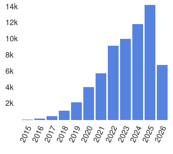
In fact, Deep Learning publications are exploding in Astronomy!
|
Figure 5. Number of refereed astronomy papers containing the text "Deep Learning" in their abstracts (~66.3K). (From NASA ADS) |
Some notable examples
Galaxy Classification
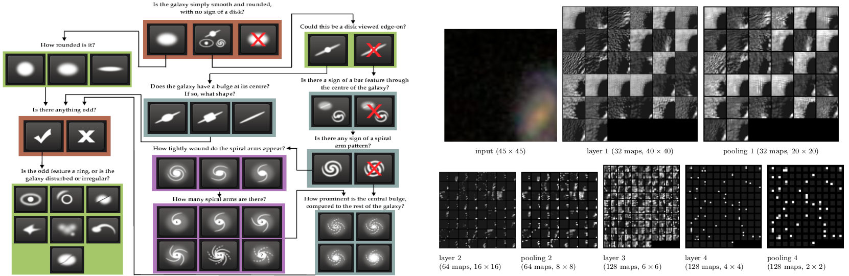
Dieleman et al. (2015), MNRAS, 450, 1441 \(-\) calculate probabilities for the 37 Galaxy Zoo possible answers
training: classification of 61,578 JPEG images from SDSS with GZ labels
architecture: standard CNN
|
Figure 6. Left $-$ Galaxy Zoo classification tree (From Willet et al. 2013). Right $-$ Activation of the CNN layers (From Dieleman et al. 2015). |
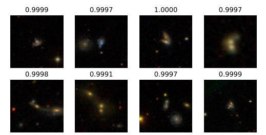
Ackerman et al. 2017, MNRAS, 479, 415 \(-\) identify mergers
training: classification of ~4000 JPEG images from SDSS with GZ labels
architecture: CNN with transfer learning
|
Figure 7. Some galaxy pairs confidently identified as mergers. (From Ackerman et al. 2017) |
Galaxy Morphology
Aragon-Calvo et al. 2020, MNRAS, 498, 3713 \(-\) obtain structural parameters via self-supervised learning
training: re-produce parameters used to generate artificial galaxies
architecture: semantic autoencoder

|
Figure 8. Fitting of morpological structural parameters with an Autoencoder. (From Aragon-Calvo et al. 2020) |
Serendipitous Detection
Lanusse et al. 2018, MNRAS, 473, 3895 \(-\) spot gravitational lenses
training: 20,000 LSST-like observations
architecture: CNN + ResNet

|
Figure 9. Some images correctly identified as hosting lenses. (From Lanusse et al. 2018) |
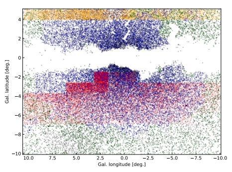
Dekany & Grebel al. 2020, ApJ, 898, 46 \(-\) spot fundamental-mode RR Lyrae stars
training: 10\(^7\)\(-\)10\(^8\) near-IR photometric time-series
architecture: RNN
|
Figure 10. Spatial distribution of the objects used as training set. (From Dekany & Grebel al. 2020) |
Image Reconstruction
Schawinski et al. 2017, MNRAS, 467, 110 \(-\) image denoising
training: 4550 nearby SDSS galaxies
architecture: GAN

|
Figure 11. Degraded image details reconstructed by a GAN. (From Schawinski et al. 2017) |
Cosmological Simulations
Rodríguez et al. 2018, ComAC, 5, 4 \(-\) create computationally cheap cosmological simulations
training: 10 independent L-PICOLA simulation boxes
architecture: GAN

|
Figure 12. Comparison between the results of a N-body simulation (left) and from a GAN (right). (Adapted from Rodríguez et al. 2018) |
Source Density Predicition
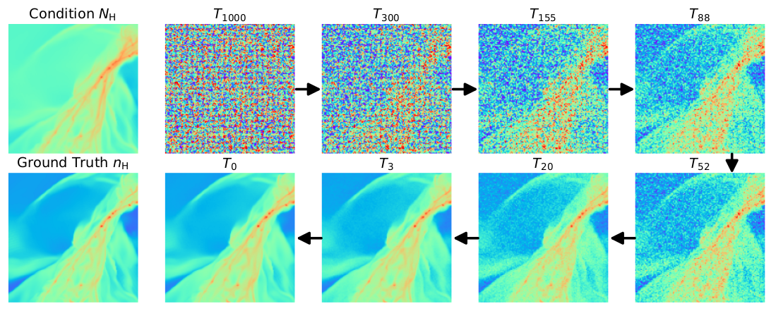
Xu et al. 2023, ApJ, 950, 2 \(-\) get a census of Giant Molecular Clouds (GMCs) from their \(N_H\) column-density images
training: 7179 high-res MHD simulations of clouds
architecture: Diffusion Models
|
Figure 13. The true GMC number density (bottom-left) is iteratively reconstructed, conditioned on the line-of-sight $N_H$ column density (top-left) . (From Xu et al. 2023, ApJ, 950, 2) |
Inference of Cosmological Parameters
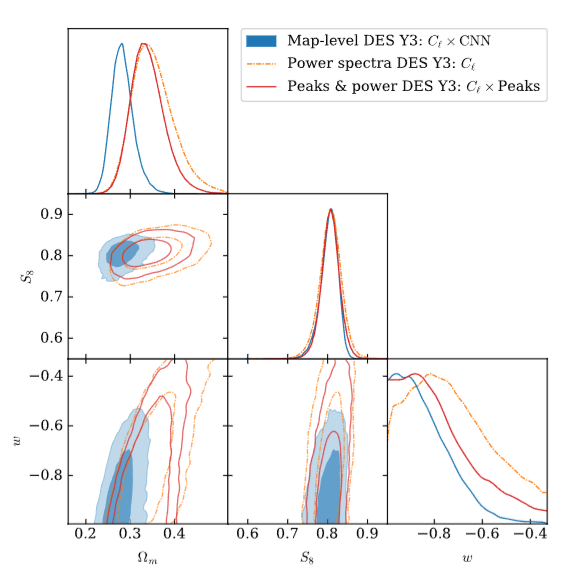
Jeffrey et al. 2025, MNRAS, 536, 2 \(-\) constrain \(𝑤\)CDM cosmological parameters using SBI on Dark Energy Survey weak-lensing maps
training: 791 full-sky \(N\)-body simulations
architecture: Simulation Based Inference + NN compression
|
Figure 14. Corner plot of the posteriors for Ωm, S8, and w. (From Jeffrey et al. 2025) |
Neural Networks (NN) Components#
Generic Architecture and Neurons#
|
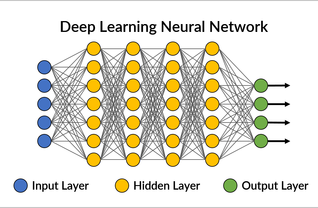
Figure 15. A simple, generic feedforward deep neural architecture. Neurons of a layer might be connected to al the neurons of the neighboring layers, like in this example (fully-connected layers), or not. (Adapted from here) |
Nomenclature
Neuron: A simple element in a network, carrying 1 value.
Layers: A collection of neurons activated simultaneously.
Layers are represented differently depending on the architecture.
E.g., fully-connected layers (as in the Figure above), appear as vertical stripes of neurons.
input layer: the data
hidden layers: the internal layers (”hidden” from the point of view of the NN user)
output layer: the variable(s) of interest (e.g., class(es) or \(y\))
E.g., if we provide an image as input, each pixel is 1 neuron of the input layer.
Contemporary NNs contain hundreds to thousands of layers, with millions to billions of neurons.
Weights and Biases#
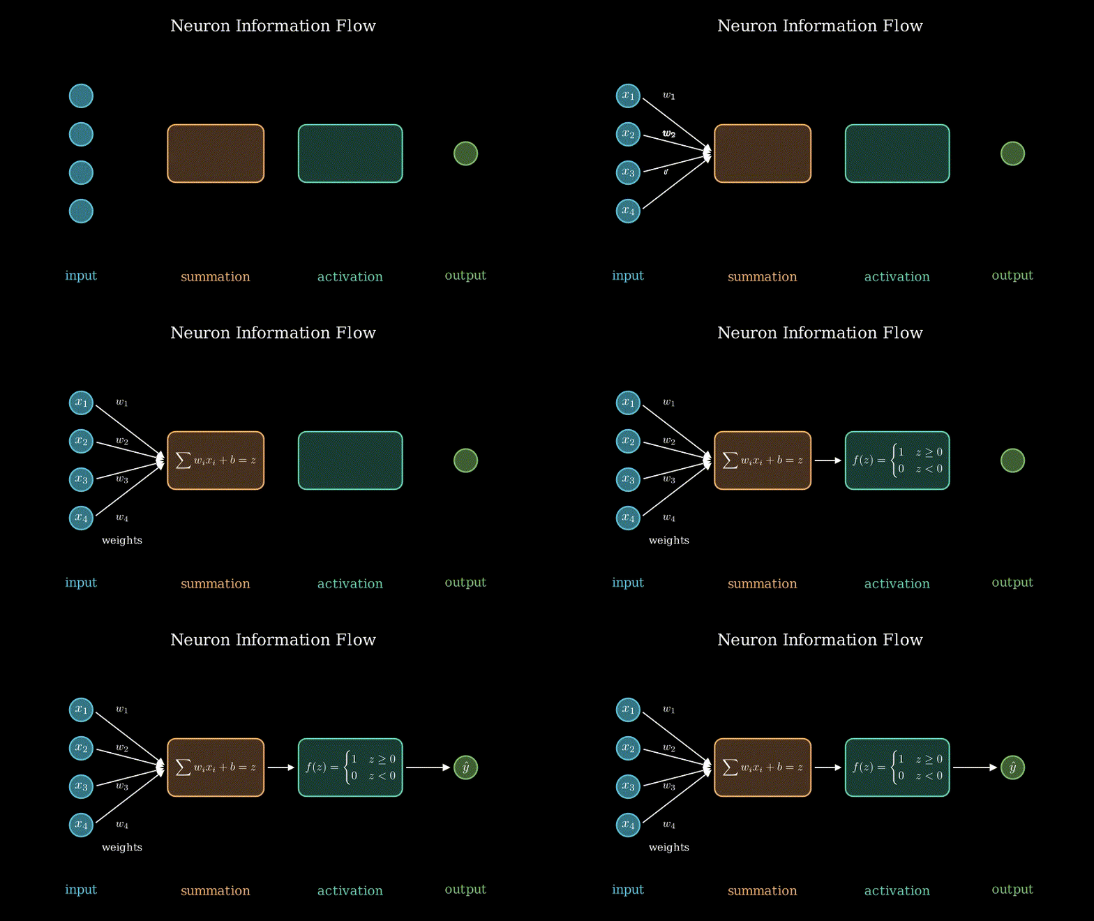
The core of the functioning of any NN is how the information flows through a neuron.
|
Figure 16. How the information is propagated through a neuron. (Image by P. Bonfini, Astrostatistics in Crete, made with Manim, free reproduction) |
The first stage is linear:
A neuron takes all the inputs (values) x\(_i\) directed into it, multiplies each of them by a different weight (\(w_i\)), and takes the sum.
Then, it adds a bias (\(b\)).The second stage is (usually) non-linear:
The summation is passed to an activation function.
The activation function acts as a filter, basically deciding when and how the information shall flow.
The ouput of a single neuron is therefore:
IMPORTANT
The weights and biases are the elements that are fit during the training of the model!
Fitting a model == optimizing all the weights and biases within the NN, in order to approximate the desired output \(y\) given a corresponding example \(x\).
Activation Functions#
Activation functions are what make NNs so efficient as universal tools.
They introduce non-linearities \(\rightarrow\) a NN can create an arbitrarily complex model.
They can be basically any filter-like function, but they better posses [some of] these features:
computationally inexpensive \(\leftarrow\) hence simple, since they get executed at each neuron
zero-centered \(\leftarrow\) not to shift values towards a preferential direction
differentiable \(\leftarrow\) because NNs work with Backpropagation
avoid vanishing when chained \(\leftarrow\) more correctly, we need to avoid vanishing gradients
(see Gradient Descent and Loss, and Glorot & Benjo 2010)
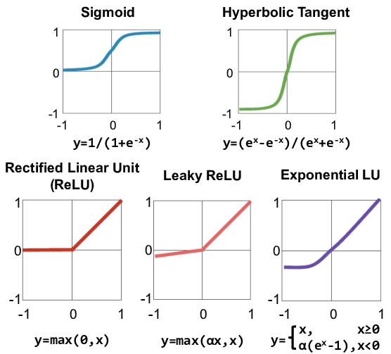
|
Figure 17. A collection of commonly used activation functions (Adapted from here) |
NN Architecture Variants#
NN come in countless architectures, and even trying to classify them is a tough task …
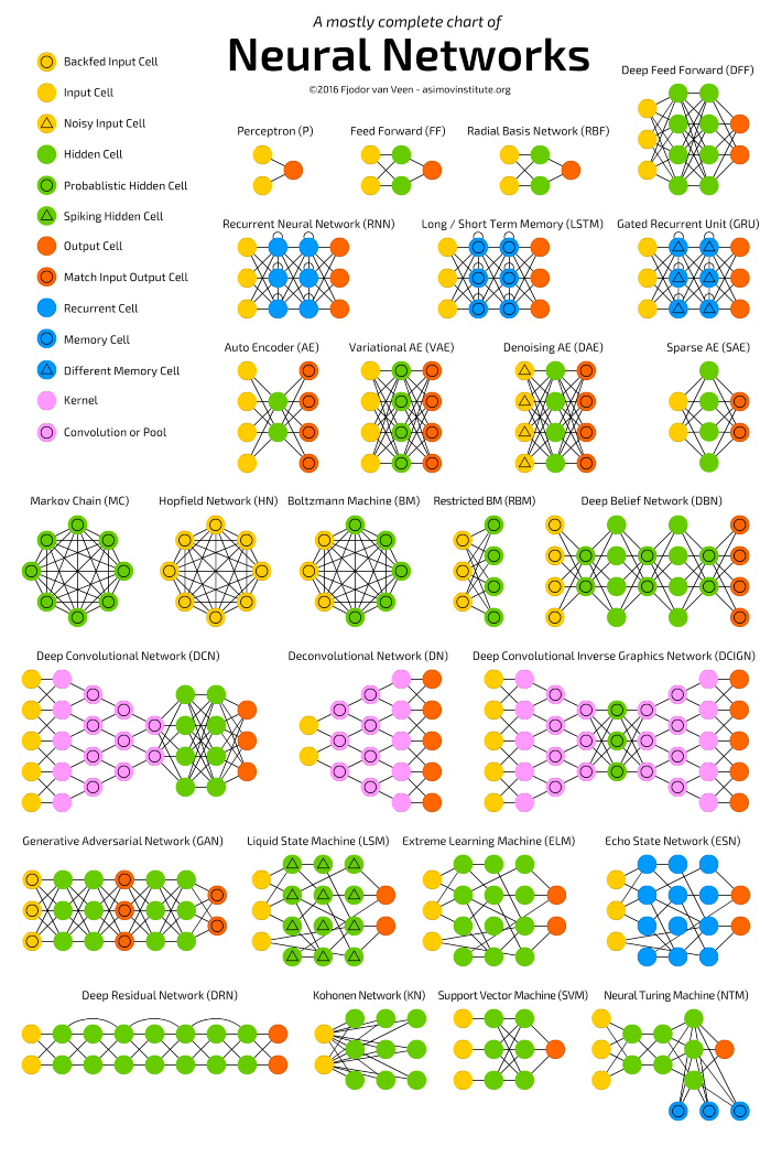
|
Figure 18. A reasonably complete scheme of basic NN architectures. (Image credit: Fjodor van Venn) |
Training NNs#
As mentioned above:
training a NN = optimize its weights and biases
in order to produce the desired output (class or values) given a corresponding input.
The details of the training method depends on the DL learning problem:
supervised: we have labelled examples
unsupervised: no labeles are available
reinforced: the examples are associated to a “reward”
In this notebook, we will focus on the supervised case to illustrate the NN mechanics:
\(\rightarrow\) Let’s assume we have some predicting variables \(X\), and labels \(y\).
How can we tell the network in which way it shall modify weights (and biases)?
Let’s break down the NN rationale:
We initialize the weights to some arbitrary value
We take a sub-sample (batch) of the data \(X\), \(X_{batch}\)
We propagate \(X_{batch}\) through the network, obtaining a predicted \(\hat{y}_{batch}\)
We assess the error between \(\hat{y}_{batch}\) and the true \(y_{batch}\)
We need to backpropagate back the information about the difference
We need to update the weights in the right direction
Repeat from step 2 untill all data are used
(Repeat from 2 for multiple epochs)
The critical steps are #4, #5 and #6.
Error Function, Gradient Descent and Backpropagation#
Let’s consider an errorr (a.k.a. loss, or cost) function:
which assesses the intensity of the error. For example, we might adopt: \(E (\hat{y}, y) = {1\over2}(\hat{y} - y)^2 \).
To be precise, \(\hat{y}\) is itself a function of the input \(\boldsymbol{x}\), and of the NN parameters \(\theta\) (all the \(w\) and \(b\) of each node):
therefore:
Our objective: Minimize the error by finding the optimal set \(\hat{\theta}\), i.e.: $\( \hat{\theta} = \min_{\theta} E(\boldsymbol{x}, y, \theta) \)$
A useful consideration
The gradient of \(E\) with respect to \(\theta\), i.e. \(\nabla_{\theta} E (\boldsymbol{x}, y, \theta)\), is a vector roughly pointing towards the minimum of \(E\):
import matplotlib.pyplot as plt
import numpy as np

def E(theta): return theta**2
def dE_dtheta(theta): return 2*theta

thetas = np.linspace(-10, 10, 400)
theta = -9
'''First guess for the parameter''';
eta = 0.18
'''Learning rate: try to change this to small/large values (e.g., 0.08, or 1)''';

plt.figure(figsize=(8, 4))
plt.title('Gradient Descent')

plt.plot(thetas, E(thetas), c='grey', lw=3, zorder=-1)

for i, color in enumerate(['C0', 'C1', 'C2', 'C3']):
    plt.scatter(theta, E(theta), s=100, c=color, label=r'$\theta$'+str(i))
    #
    theta_prime = theta - eta*dE_dtheta(theta)
    plt.arrow(theta, E(theta), theta_prime - theta, 0, lw=3, head_width=2, head_length=0.2, fc=color, ec=color, length_includes_head=True)
    plt.plot([theta_prime, theta_prime], [E(theta), E(theta_prime)], '--', lw=3, c='darkgrey', zorder=-1)
    plt.text((theta + theta_prime) / 2, E(theta) + 1, r'$\nabla_{\theta} E$', ha='center', va='bottom')
    #
    theta = theta_prime

plt.gca().spines['top'].set_visible(False)
plt.gca().spines['right'].set_visible(False)
plt.xlabel(r'$\theta$', fontsize=14)
plt.ylabel(r'E($\theta$)', fontsize=14)
plt.legend(loc='upper left', bbox_to_anchor=(1,1))
plt.show()
We can therefore update the weights by adding a vector proportional to \(\nabla_{\theta} E\):
where the proportionality constant \(\eta\) is called learning rate (LR) because it regulates how fast we shall proceed towards the mininum
(and possibly overshoot it, if \(\eta\) is too large).
This is the Gradient Descent optimization.
In-class Exercise [5 min]: In the above code block, try to change the value of eta to see what happens when the update is too fast or too slow
Calculating the gradient
We have \(\nabla_{\theta} E~\):
where the \(\theta_i\) are all the weigths and biases along the network.
.. BUT … how do I exactly calculate each \(\frac{\partial E}{\partial \theta_i}\) ?
For example, consider the simple network:
2 input neurons
2 hidden layers, each with 2 neurons
2 output neurons
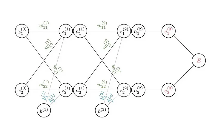
|
Figure 19. All the parameters of a 2-hidden-layer NN. (From this amazing graphical explanation by Brent Scarff) |
where, in this notation:
\( z = \sum{\textbf{w}\cdot{}\textbf{x} + b} \)
is just the neuron value before the activation function\( a = f(z) \)
is just the neuron value after the activation function
How do I calculate, e.g.: $\( \frac{\partial E}{\partial w^{(2)}_{11}} ~~~~~ ?\)$
\(\rightarrow\) Chain rule of derivatives !

Figure 20. Calculating the gradient at a specific position in the NN. (Image credit: Brent Scarff) |
We can just apply the same trick over and over, to get any component of \(\nabla E_\theta\):

|
Figure 21. Calculating the gradient at a deeper position in the NN. (Image credit: Brent Scarff) |
You can imagine propagating the chain rule back to the original input: all the steps are either linear or passing through a differentiable activation function!
With that, we now how to update any \(w\) and \(b\):
This is the Backpropagation technique.
[-] Strongly suggested read: This blog by Brent Scarff.
Optimization Algorithms [optional]#
Let’s recall Equation 1:
Ok \(-\) we have the Gradient method \(-\) BUT:
A NN model can easily contain millions of parameters \(\rightarrow\) Can we efficiently explore the parameter space, to find the global minimum?
How do we pick the correct learning rate \(\eta\) ?
\(\rightarrow\) Optimization Algorithms address these issues.
Momentum optimization#
This method takes in account the previous values of the gradient.
It is particularly useful when exploring monotonic parameter spaces, because it can skip faster through large areas of the landscape.
The parameter update is a variation to Equation 1:
\(\beta\) represents the current “velocity” of the gradient.
The larger \(\beta\in\) [0, 1], the more previous steps are taken into account.
We can interpret Equation 2 as:
“Globally descending following the direction m, and updating m based on local gradient.”

|
Figure 22. Representation of the influence of Momentum on the GD. The descent is much faster than the standard Gradient Descent (i.e. $\beta = 0$) However, for very large values of $\beta$, the search can 'oscillate' around the optimum point. (From here) |
Adaptive learning rates#
They address the issue that the descent is different for each parameter (i.e., for each ‘direction’ in the parameter space):
Their differ on how they dynamically adjust the learning rate (LR).
AdaGrad
AdaGrad separately scales the LR for each parameter \(\rightarrow\) Each direction gets a “personalized” search.
LR scaling \(\leftarrow\) inversely to the sum of the squares of all the historical gradients.

|
Figure 23. AdaGrad optimization compared to that of Gradient Descent. (Adapted from Figure 11-7, A. Gerone 2022) |
PROs:
Directions with larger gradient see their LR decrease faster.
MAJOR CON:
May stop too early \(\rightarrow\) better not use it!
RMSProp
Puts a patch to AdaGrad early stopping.
LR scaling \(\leftarrow\) inversely to the exponentially weighted moving average of previous gradients.
Adam
Adam (i.e., Adaptive Moments) is sort of RMSProp + Momentum Optimization.
LR scaling \(\leftarrow\) uses both the first and the second moment of past gradients.
NOTE: Don’t confuse “moment” of a quantity with “momentum”:
moment_1 = average
moment_2 = uncentered variance (variance without centering around the mean)
In other words, RMSProp uses the first moment \(-\) with \(E[]\) being an exponentially-weighted average.
Adam also makes use of the second moments of the historical gradients.
TL;DR: Adam is arguably the best-performing optimizer on average:
quite robust with respect to the choice of hyperpars
usually works with default hypepars
\(\rightarrow\) Safe choice!
Reading material
At this page you will find graphical explanations of these [and more] optimizers as well as their mathematical formulations.
Learning Curves#
In DL, it is common to cycle the training on the same data \(N\) times \(-\) Each pass is called “Epoch”.
Training rationale with N_epochs epochs, and N_batches batches:
0. set epoch = 0
1. Train on batch 1, update gradient
   Continue train on batch 2, update gradient
   Continue train on batch 3, update gradient
   .. .
   Continue train on batch N_batches, update gradient
3. epoch += 1
   (epoch completed)
4. if epoch <= N_epochs: continue from 1 else stop
NOTE: This introduces bias towards the training data, but it usually more than compensated by a longer gradient descent.
We can display the values of the Loss as a function of “time” \(\rightarrow\) Learning Curves (Validation Curves)

|
Figure 24. Learning curves for train and validation set. (From here) |
We can use them to spot overfitting (train goes much better than validation) or underfitting (training shows trend to improve):

|
Figure 25. Learning curves for train and validation set. |
| Underfitting | A good fit | Overfitting |
|---|---|---|
| The training set shows a downward trend at the right edge: maybe a few more epochs could yield a better performance. |
Training and validation converge and they flatten. |
The validation curve cannot keep up with the training curve. |
What you will see in the Workshops#
You will explore 2 applications of DL networks:
Supervised Learning - Regression \(~~~~\rightarrow\) Fully-connected Layers
Supervised Learning - Classification \(~\rightarrow\) Convolutional Neural Networks (CNNs)
Supervised Learning: A simple Deep NN#
We will enter the DL coding realm via a simple Regression problem.

|
Figure 26. The struggle of Regression. (Adapted from xkcd) |

|
Figure 27. A simple Deep NN can be used as a regressor. (From here) |
Supervised Learning: CNNs#
CNNs excel at classifying images thanks to their Convolutional Layers:

|
Figure 28. A prototypical CNN architecture. |
Convolution \(~\rightarrow\) Filters that scan the image to detect different features
Pooling \(~~~~~~~~\rightarrow\) Reduce dimensionality to increase abstraction
Flattening \(~~~~\rightarrow\) Encodes features into variables
Dense Layers \(\rightarrow\) Feature classifier
Libraries#
There are several libraries that implement Deep Learning routines in Python.
For the Woskshops we will focus on Tensorflow (\(\rightarrow\) via Keras), and Pytorch.
TensorFlow#

TensorFlow (Google) does the heavy lifting for us:
pre-defined functions and layers
automatically computes the derivatives (for Backprop!)
TensorFlow via Keras#
Keras is an API (Application Programming Interface) \(-\) it provides higher-level functionalities for DL libraries, e.g.:
Tensorflow
Pytorch
JAX
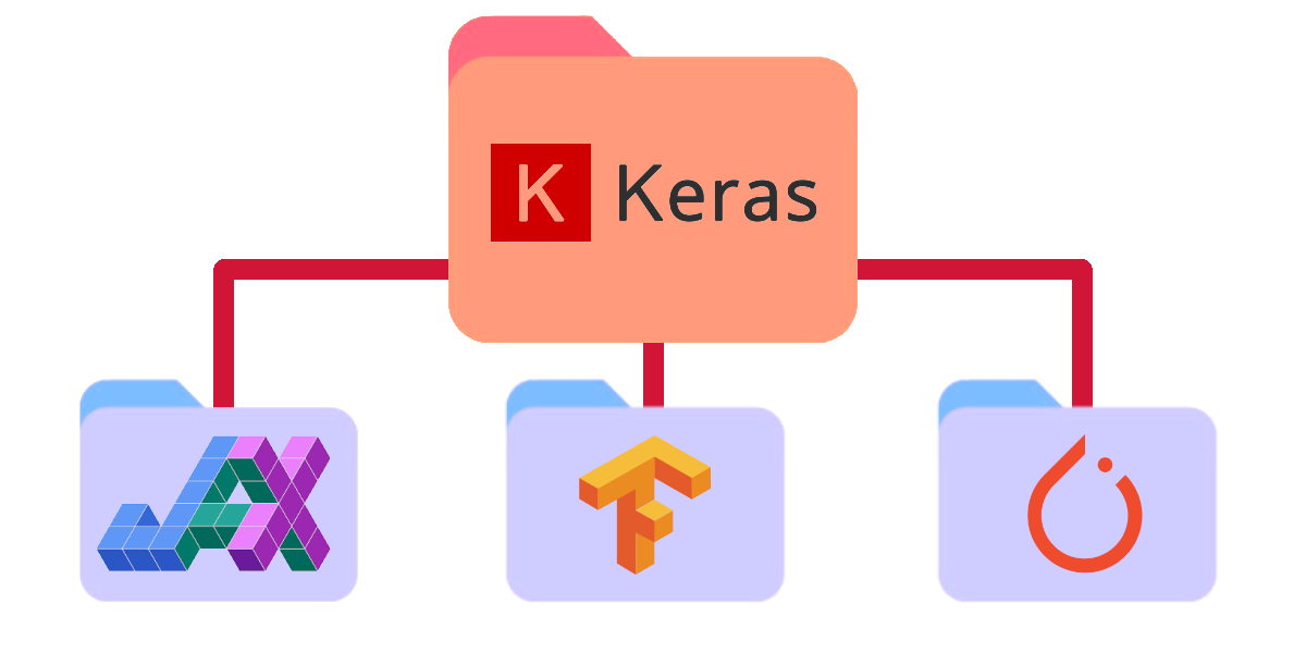
You can see it imported in different ways, because it is mantained separately by both Tensorflow and Keras (functionalities might differ slightly):
# Install: Anaconda -> Tensorflow -> Keras
#
import keras.models
# and
from keras import backend as K
# use Keras repository code

# ... OR

import tensorflow.keras
# use TensorFlow repository code itself (recommended: better maintained)

"""NOTE: Importing Keras usually results in several warnings.  Do not be scared.""";
Keras can be coded in 2 main “styles”:
Sequential API#
PROs: Simpler (stack of layers)
CONs: Single-input, single-output
import tensorflow.keras as keras
from keras import layers
import tensorflow as tf
tf.config.set_visible_devices([], 'GPU')  # Just to bypass potential GPU issues

# Either:
model = keras.Sequential(name="Sequential Example")
model.add(layers.Dense(20, activation='relu'))
model.add(layers.Dense(10, activation='softmax'))

# ... OR:
model = keras.Sequential([
    keras.layers.Dense(20, activation='relu', input_shape=(7,)),
    keras.layers.Dense(10, activation='softmax')
], name="Sequential Example")

model.summary()
#model.fit(x_train, y_train, epochs=5, batch_size=32)
Functional API#
PROs: More flexible, multi-input, multi-output
CONs: Steep learning curve, need to understand tensor programming
import tensorflow.keras as keras
from keras import layers
import tensorflow as tf
tf.config.set_visible_devices([], 'GPU')  # Just to bypass potential GPU issues

inputs = keras.Input(shape=(7,))
x = layers.Dense(20, activation='relu')(inputs)
outputs = layers.Dense(10, activation='softmax')(x)

model = keras.Model(inputs, outputs, name="Functional Example")
model.summary()
#model.fit(x_train, y_train, epochs=5, batch_size=32)
Pytorch#

Pretty much the same concept:
Sequential API
Functional API
Let’s see the Functional API, which in Pytorch is istantiated as a class.
Functional API#
import torch
import torch.nn as nn
import torch.nn.functional as F

class MyModel(nn.Module):
    def __init__(self):
        super(MyModel, self).__init__()
        self.fc1 = nn.Linear(7, 20)
        self.fc2 = nn.Linear(20, 10)

    def forward(self, x):
        x = F.relu(self.fc1(x))
        x = F.softmax(self.fc2(x), dim=1)
        return x

# Instantiate the model:
model = MyModel()
print(model)
###EOF