
Basics of Optimization#
This notebook introduces to the concept of “optimization”, in the sense of finding the best parameters of a function.
Notice that “optimization” is an umbrella term, which, depending on the specific context, can manifest as:
minimization
maximization
fitting
In this notebook, we will focus on function fitting, but the concepts outlined here are valid for optimization in general.
For the sake of this school, we can use the terms “fit” and “optimize” interchangeably
Setup#
# in case it is not installed, eg Google's Colab
%pip install lmfit --quiet
import numpy as np
import pandas as pd
import matplotlib.pyplot as plt
import seaborn as sns
import requests

from IPython.display import display, HTML
display(HTML("<style>.container { width:100% !important; }</style>"))


url = "https://raw.githubusercontent.com/AstroStat-Academy/assets-public/main/colab/clone_and_cd_colab.py"
colab = requests.get(url).text
exec(colab)

url = "https://raw.githubusercontent.com/AstroStat-Academy/assets-public/main/styles/plot_style.py"
style = requests.get(url).text
exec(style)
Running locally, skipping Colab setup.
Imported matplotlib.
Imported seaborn.
Plotting style set.
What is [parametric] fitting#
Easiest to start with a linear example.
Say we have some observed data:
X = [1, 2, 3, 4, 5]
y = [0.2, 0.4, 0.5, 0.8, 0.9]

from matplotlib import pyplot as plt
plt.figure(figsize=(3,3))
plt.scatter(X, y)
plt.show()
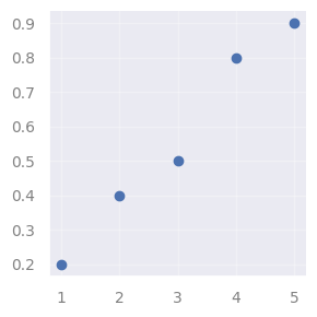
… and we want a model that represents the true behavior of the data.
We may want to use it for:
predicting new data
explain the phenomenon that causes our observations
Let’s assume a one-dimensional linear model, that is, a model of the type:
where we call \(\alpha\) and \(\beta\) the model parameters.
By changing the parameters we obtain different models, e.g.:
import numpy as np

def funct(xx, alpha, beta):
    return alpha*xx + beta

xx = np.linspace(0 ,5, 100)
'''Notice that `xx` is not the same as `X` (the data), but just
an array of equally spaced values that we use for plotting purposes.'''

alphas = [0.1, 0.27, 0.05]
betas  = [0.2, -0.2, 0.3]

plt.figure(figsize=(3,3))

for i, (alpha, beta) in enumerate(zip(alphas, betas)):

    y_model_i = funct(xx, alpha, beta)
    plt.plot(xx, y_model_i, label='model %s' % i, c=str('C%s' % (i+1)))

plt.scatter(X, y)
plt.legend()
plt.show()
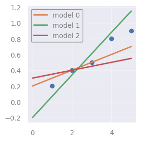
It is convenient to think that each parameter set gives rise to a different model
(\(\rightarrow\) convenient for when we will talk about “model selection”)
So the problem of picking the best-fitting model becomes \(\rightarrow\) How do I pick the best \(\alpha\) and \(\beta\)?
Q: First of all: what “best” means? (in-class discussion)
[Spoiler]
\(\rightarrow\) We need to define a metric of fitness!
As a fitness metric, we could use the error that each model makes. For each observed datum, the error is:
where \( \hat{y}_i\) is the model prediction for the corresponding \(x_{i}\):
plt.figure(figsize=(3,3))

yhat_1 = funct(np.array(X), alphas[1], betas[1]) # model predictions (dots)
y_model_1 = funct(xx, alphas[1], betas[1]) # just for plotting the model (line)

plt.plot(xx, y_model_1, c='C2')
errs = plt.plot((X, X), (y, yhat_1), c='grey', label='err')
plt.setp(errs[1:], label="_")
plt.scatter(X, y, label='y', c='C0')
plt.scatter(X, yhat_1, label=r'$\hat{y}$', c='C2')

plt.scatter(X, y)
plt.legend()
plt.show()
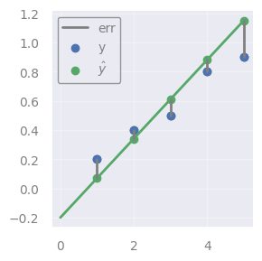
\(\rightarrow\) So what about picking the \(\alpha\) and \(\beta\) that minimize the errors?
It’s easier if we minimize a single number, so, we can consider the “sum of errors”:
Q: But minimizing this has a problem. Can you guess? (in-class discussion)
[Spoiler]
\(\rightarrow\) The problem here is that positive and negative errors can actually cancel out - resulting in a misleading concluion regarding the performance of the method.
We consider the sum of squares:
and hence the Least Squares Method:
The best-fitting parameters (=model) are those that minimize the sum of squares of the errors
IMPORTANT:
The Least Squares method is only one possible optimization method.
As we will see over and over again during this school, there are other definitions of “best fitting model” (e.g. the one that minimizes the absolute error), as well as countless algorithms to find such optimum.
Yet, LS is a very good example to start with, to get the general intuition behind optimization.
Fitting a line via Ordinary Least Squares (OLS)#
The linear case offers the simplest application of LS fitting, which goes under the name of Ordinary Least Squares (OLS).
Simple \(\rightarrow\) We can solve this analytically (no approximations, no iterations, computationally fast).
Problem definition#
We follow this wikipedia article on OLS for the formalism/nomenclature.
We first need to generalize to \(p\) dimensions \(\rightarrow\) now, each \(X_i\) for sample \(i\) is not a single feature (as before), but an array of features:
So, if we have \(n\) samples, each having \(p\) dimensions, the data matrix is:
NOTE: Samples are along rows, in this notation.
However, the target variable is still one-dimensional:
Now, for the model \(-\) In the 1D cases we said it was:
Generalizing to \(p\) dimensions, one could say that the multi-dimensional model should be of the form:
… where “const” plays the role of \(\beta\) in the 1D case, and instead of using \(\alpha\), \(\beta\), \(\gamma\), etc., we just use \(\beta_1\), \(\beta_2\), \(\beta_3\), not to run out of Greek letters!
We can forget about the const with a small trick, without losing generalization (again, see the wikipedia OLS article) \(-\) so our generalized multi-dimensional linear model becomes:
But, to be formally precise, we should add the index \(i\), because this must hold true for every data point \(i\):
or, in vector notation:
for each point \(i\). In matrix notation we can represent the equations for all points in one go:
[Solution]
See this wikipedia article on Least squares for the derivation.
The solution is obtained by:
Writing the squares in a convenient form
Finding the minimizer by searching where the derivative of \(S(\pmb{\beta})\) equals 0
IMPORTANT: We want to minimize \(S(\pmb{\beta})\) with respect to \(\pmb{\beta}\), not \(\pmb{X}\) !
\(\rightarrow\) i.e., we are looking for the best parameter set \(\hat{\pmb{\beta}}\) that minimizes the squared errors:\(\pmb{\hat{\beta}} = \operatorname{argmin_\beta} S(\pmb{\beta})\)
simplifying, and moving terms around it follows:
Extremely simple
But is it computationally fast?
Inverting a matrix (in our case, (\(\pmb{X}^T\pmb{X})^{-1}\)) is a “heavy lifting” job for a computer.
\(\rightarrow\) complexity: \(\mathcal{O}(n^3)\)
In python#
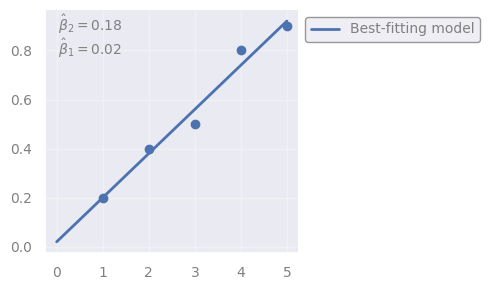
We will use numpy.linalg.lstsq to fit:
to the data seen above (notice that now we call every parameter as “\(\beta_{<number>}\)”, as for the generic multi-dimensional case).
# Same data as above:
X = np.array([1, 2, 3, 4, 5])
y = np.array([0.2, 0.4, 0.5, 0.8, 0.9])

from numpy.linalg import lstsq

X_prime = np.vstack([X, np.ones(len(X))]).T
'''
What is this line doing?! Adding a row of `1`s to our data?! Why?

Remember, above, when we said that we can "hide" the constant in:
    y = beta*X + const
using a trick?

The trick it is to create a "fake", additional feature in X, and fill it
with ones.  This will play the role of the constant.

See the links above, as well as the `np.linalg.lstsq` documentation, here:
    https://numpy.org/doc/stable/reference/generated/numpy.linalg.lstsq.html
''';

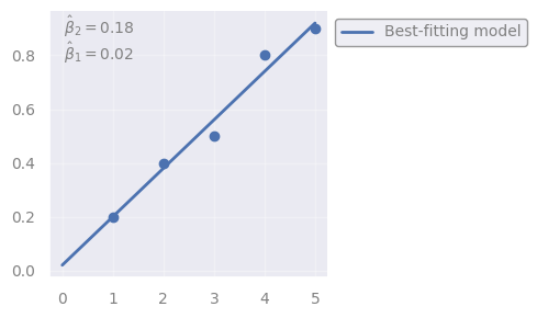
beta_2_hat, beta_1_hat = np.linalg.lstsq(X_prime, y, rcond=None)[0]
# best-fitting parameters

fig, ax = plt.subplots(figsize=(5,3), ncols=1, nrows=1)
plt.scatter(X, y)
plt.plot(xx, beta_2_hat*xx + beta_1_hat, 'C0', label='Best-fitting model')
plt.text(.05, .99, '$\\hat{\\beta}_2 = %.2f$' % beta_2_hat, ha='left', va='top', transform=ax.transAxes)
plt.text(.05, .89, '$\\hat{\\beta}_1 = %.2f$' % beta_1_hat, ha='left', va='top', transform=ax.transAxes)
plt.legend(bbox_to_anchor=(1, 1))
plt.show()
In python - an easier library#
Ok, numpy.linalg.lstsq is very educational because it solves the OLS problem algebraically, just like in Equation 1.
But \(-\) as you have seen \(-\) it has a clumsy usage.
For practical purposes, we will now on use the much more intuitive and flexible lmfit.
NOTE: Internally, it uses by default a different algorithm to solve the least-squares problem (see later: “Levenberg-Marquardt”), but we pretend not, for now.
from lmfit import Model

def model_func(x, beta_1, beta_2):
    y = beta_2*x + beta_1
    return y

# Create an lmfit `Model` object:
model = Model(model_func)

# Invoking the `fit()` method, which returns the object `result`:
result = model.fit(y, x=X, beta_1=0, beta_2=1)
'''
Notice that here we are providing some initial guess for `beta_1` and `beta_2`,
this is only because this library is using the Levenberg-Marquardt algorithm.

In reality OLS doesn't need initial guesses when using the algebraic solution,
as demonstrated above by using `np.linalg.lstsq`, which properly solves OLS.

We will see later why Levenberg-Marquardt requires initial guesses.
'''

# Retrieving best-fit parameters:
beta_1_hat = result.params['beta_1'].value
beta_2_hat = result.params['beta_2'].value

xx = np.linspace(0 , np.max(X), 100)
'''Notice that `xx` is not the same as `X` (the data), but just
an array of equally spaced values that we use for plotting purposes.'''

fig, ax = plt.subplots(figsize=(5,3), ncols=1, nrows=1)
plt.scatter(X, y)
plt.plot(xx, beta_2_hat*xx + beta_1_hat, 'C0', label='Best-fitting model')
plt.text(.05, .99, '$\\hat{\\beta}_2 = %.2f$' % beta_2_hat, ha='left', va='top', transform=ax.transAxes)
plt.text(.05, .89, '$\\hat{\\beta}_1 = %.2f$' % beta_1_hat, ha='left', va='top', transform=ax.transAxes)
plt.legend(bbox_to_anchor=(1, 1))
plt.show()
/home/grigoris/miniconda3/envs/astrostat25/lib/python3.12/site-packages/uncertainties/core.py:1024: UserWarning: Using UFloat objects with std_dev==0 may give unexpected results.
  warn("Using UFloat objects with std_dev==0 may give unexpected results.")
Exercise 1 [15 min]
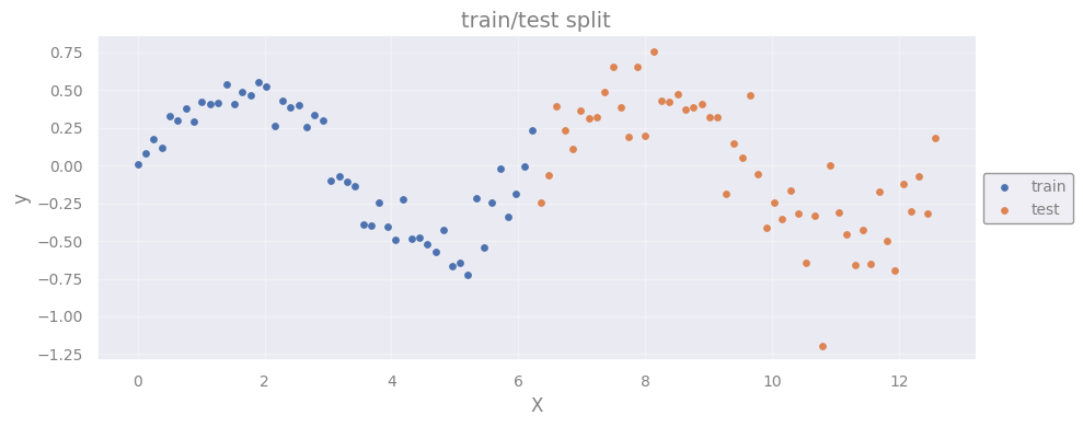
Objective: Evaluate the best-fit model to some data. You will have to assume a model, and then run the Least-Squares minimization on the provided data.
The final goal is to observe what happens when you apply the model to new, “test” data.
Dataset: The following one.
Task: In particular, you will have to:
Look at the data and assume a model
Use only the “train” data to perform the LS minimization to find the best model
Using the best model, calculate and plot the model predictions on the “train” data
Calculate and plot the model predictions on the “test” data
Calculate the squares of errors for the “train” (\(S_{train}\)) and “test” (\(S_{test}\)) data
Now compare the two squares of errors \(\rightarrow\) What do you notice?
Hints:
For task 5 \(-\) To get the squares of errors you can simply calculate: $\( S_{train} = \sum_i (y_i - \hat{y}_i)^2 ~~~~~ \forall i \in train\)$
Notice that \(-\) once the model has been fit \(-\) \(S_{train}\) is effectively the minimized Least Squares.
But what about \( S_{test} \)?
# Loading and plotting data:
import tarfile
import io
from matplotlib import pyplot as plt
import numpy as np

tar = tarfile.open("data/data_inclass_ex1.tar.gz", "r:gz")

def convert_and_load(file):
    with io.BytesIO(file.read()) as f:
        return np.load(f)

for member in tar.getmembers():
    file = tar.extractfile(member)
    if member.name == 'X_train.npy': X_train = convert_and_load(file)
    if member.name == 'y_train.npy': y_train = convert_and_load(file)
    if member.name == 'X_test.npy':  X_test  = convert_and_load(file)
    if member.name == 'y_test.npy':  y_test  = convert_and_load(file)

plt.figure(figsize=(10, 4))
plt.scatter(X_train, y_train, label='train', c='C0', s=15)
plt.scatter(X_test,  y_test,  label='test',  c='C1', s=15)
plt.xlabel('X')
plt.ylabel('y')
plt.title('train/test split')
plt.legend(loc='center left', bbox_to_anchor=(1, 0.5))
plt.show()
from lmfit import Model

# 1. Assuming a sinusoidal model
def model_func( ... ):
    y = ...
    return y

# 2. Using only the "_train_" data to perform the LS minimization

# Create an lmfit `Model` object:
model = Model(...)

# Invoking the `fit()` method, which returns the object `result`:
result = model.fit(...)

# Retrieving best-fit parameters:
beta_1_hat = result.params['beta_1'].value

# 3. Calculating and plotting the model predictions on the "_train_" data
# 4. Calculating and plotting the model predictions on the "_test_" data
# Predictions of the model for train/test:
yhat_train = ...
yhat_test  = ...

xx = np.linspace(0 ,np.max(X_test), 100)
'''Notice that `xx` is not the same as `X` (the data), but just
an array of equally spaced values that we use for plotting purposes.'''

plt.figure(figsize=(10, 4))
# Data:
plt.scatter(... , ..., label='train', c='C0', s=15)
plt.scatter(... , ...,  label='test',  c='C1', s=15)
# Model:
plt.plot(xx, model_func(xx, beta_1_hat), label='model', c='grey', lw=2)
# Train predictions:
plt.scatter( ..., ..., label=r'$\hat{y}_{train}$', c='C2', s=15)
# Test predictions:
plt.scatter( ..., ...,  label=r'$\hat{y}_{test}$',  c='C3', s=15)
#
plt.xlabel('X')
plt.ylabel('y')
plt.title('Best-fitting model')
plt.legend(loc='center left', bbox_to_anchor=(1, 0.5))
plt.show()
# 5. Calculating squares of errors for the "_train_" and "_test_":
S_train = ...
S_test  = ...

# 6. Now comparing the two squares:
print("S_train: %.2f | S_test: %.2f" % (S_train, S_test))
[Solution at the end !]
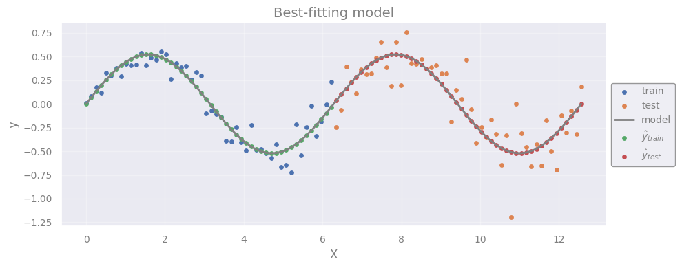
\(S_{test}\) is way larger than \(S_{train}\) \(\rightarrow\) overfitting
This is to be expected because the model has been trained on \(X_{train}\), and, as you can see, \(X_{test}\) shows larger variance.
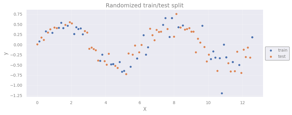
Q: What could we do to obtain a more balanced model (i.e., a model with similar performance on train and test data)? (in-class discussion)
[Spoiler]
\(\rightarrow\) Shuffle the data!
'''Merging train and test data, first.'''
X = np.concatenate((X_train, X_test))
y = np.concatenate((y_train, y_test))

'''
Now performing a random split of the merged data.
Re-running this block will generate a new, randomized split.
'''
idxs_train_ = np.random.choice(np.arange((len(X))), size=len(X_train))
# ^here we pick at random some train indexes from the merged `X`
idxs_test_ = list(set(np.arange((len(X)))) - set(idxs_train_))
# ^here we pick the complementary indexes

X_train_ = X[idxs_train_]
y_train_ = y[idxs_train_]
X_test_ = X[idxs_test_]
y_test_ = y[idxs_test_]

plt.figure(figsize=(10, 4))
plt.scatter(X_train_, y_train_, label='train', c='C0', s=15)
plt.scatter(X_test_,  y_test_,  label='test',  c='C1', s=15)
plt.xlabel('X')
plt.ylabel('y')
plt.title('Randomized train/test split')
plt.legend(loc='center left', bbox_to_anchor=(1, 0.5))
plt.show()
'''Re-running the same fit as above on the new, randomized split.'''
from lmfit import Model

def model_func(x, beta_1):
    y = beta_1*np.sin(x)
    return y

model = Model(model_func)

result = model.fit(y_train, x=X_train, beta_1=0)

beta_1_hat = result.params['beta_1'].value

yhat_train_ = model_func(X_train_, beta_1_hat)
yhat_test_  = model_func(X_test_,  beta_1_hat)

xx = np.linspace(0 ,np.max(X), 100)

plt.figure(figsize=(10, 4))
plt.scatter(X_train_, y_train_, label='train', c='C0', s=15)
plt.scatter(X_test_,  y_test_,  label='test',  c='C1', s=15)
plt.plot(xx, model_func(xx, beta_1_hat), label='model', c='grey', lw=2)
#
plt.xlabel('X')
plt.ylabel('y')
plt.title('Best-fitting model')
plt.legend(loc='center left', bbox_to_anchor=(1, 0.5))
plt.show()

S_train = np.sum( (yhat_train_ - y_train_)**2 )
S_test  = np.sum( (yhat_test_ - y_test_)**2 )
print("S_train: %.2f | S_test: %.2f" % (S_train, S_test))
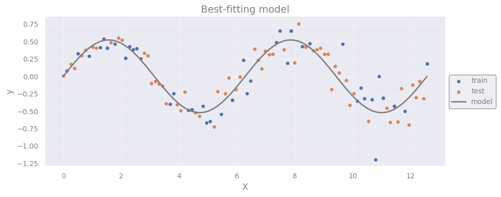
S_train: 1.96 | S_test: 1.30
Non-linear least squares: Levenberg-Marquardt algorithm#
We saw linear problems, i.e. when the model is linear in the parameters, e.g.:
What about the non-linear problems, i.e. when the model is not linear in the parameters, e.g.:
In general, LS not solvable algebraically \(\rightarrow\) Need to converge to the solution!
Brute-force approach (spoiler: doesn’t work!)#
Objective: The taks is \(-\) as usual \(-\) to find the parameter set \(\hat{\pmb{\beta}}\) that minimizes the sum of squares \(S(\pmb{\beta})\).
So, let’s say that we have a model of the type:
and we want to find \(\hat{\pmb{\beta}} = (\hat{\beta_1}, \hat{\beta_2})\) that minimizes \(S(\beta_1, \beta_2)\).
Let’s assume we could potentially explore all possible parameter combinations.
For each given \((\bar{\beta}_1, \bar{\beta_2})\) set, we:
Create a the corresponding model: \(\bar{y}_{pred} = \bar{\beta}_1e^{\bar{\beta}_2 x} \)
Calculate \(S(\bar{\beta}_1, \bar{\beta}_2) = \sum_i^{n}(\bar{y}_{i, pred} - y_{i, obs})^2\)
… and repeat ad infinitum.
\(\rightarrow\) Then, we could hypothetically map the whole \(S(\beta_1, \beta_2)\) space:
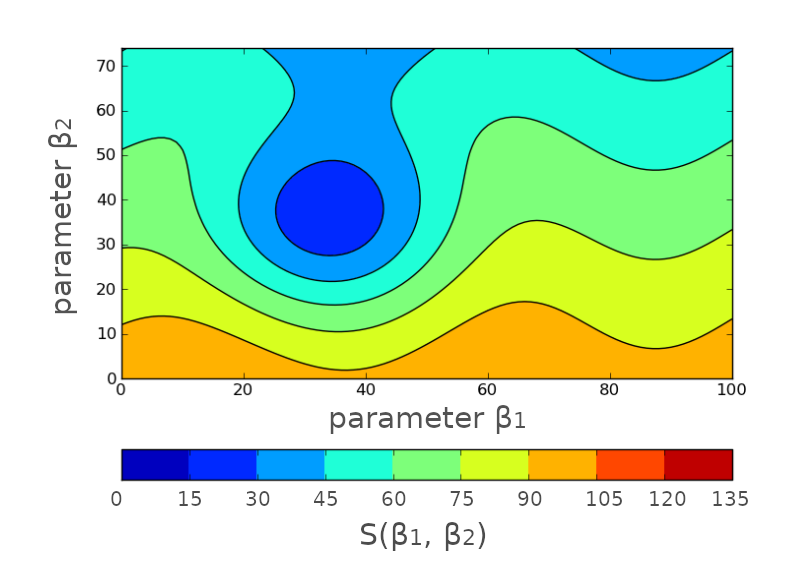
Except that this will take forever*!
*unless you have GPUs!
Iterative approach (now we are talking!)#
Instead, we may want to converge to the best solution \(\hat{\pmb{\beta}} = (\hat{\beta_1}, \hat{\beta_2})\).
(possibly in a fast way)
We will accept a compromise: approximate solution.
We start from a blank state:
Or, better, from an initial guess \((\beta^A_1, \beta^A_2)\):
(We look at the function, we had an enlightment, we used cheat codes, etc.)
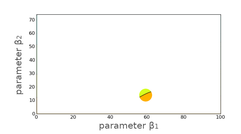
NOTE: Here we conveniently show the neighborhood around the point we pick.
Q: Where to take the next guess?
[Spoiler]
What about looking at the gradient (i.e., derivative) around that point \(\rightarrow\) it points towards where the \(S(\beta_1, \beta_2)\) is decreasing.

|
Let’s follow the white rabbit and see where it leads us …
We take the next guess \((\beta^B_1, \beta^B_2)\) somewhere along the gradient:
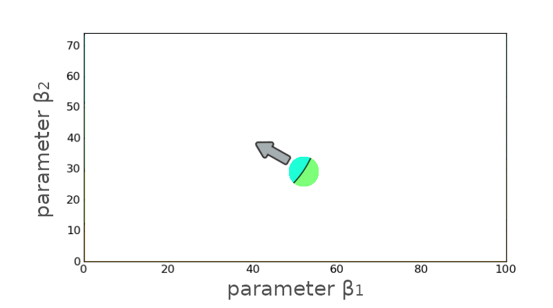
Not bad! It lead us to a lower \(S(\beta_1, \beta_2)\). Let’s try again …
We take another guess somewhere along the gradient:
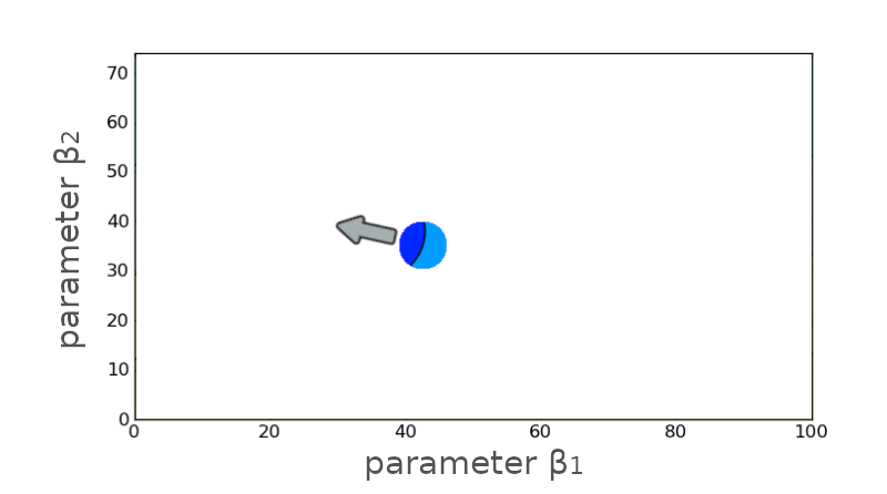
And again, and again .. until we are happy (define happy)
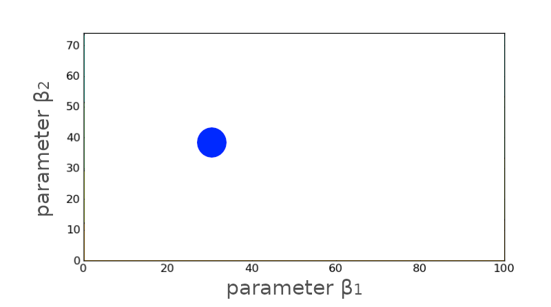
The mathematical approach#
NOTE: The theory in this section is adopted from this wikipedia article on Levenberg-Marquardt algorithm
Let’s call: \(\hat{y}_i := f(x_i, \pmb{\beta})\) \(\leftarrow\) model value for \(x_i\)
The initial guess for the best-fit parameters is \(\pmb{\bar{\beta}}\).
The next guess is: \(\pmb{\bar{\beta}}^{\prime} \leftarrow \pmb{\bar{\beta}} + \pmb{\delta}\), where \(\pmb{\delta}\) is the small amount we move by.
Objective: Update \(\pmb{\bar{\beta}}\) until we minimized \(S(\pmb{\beta})\)
[The math details]
We can use the Taylor expansion to approximate \(f(x_i, \pmb{\bar{\beta}}^{\prime})\) around \(\pmb{\bar{\beta}}\):
IMPORTANT: Notice that the derivative is on the parameters (\(\pmb{\beta}\)), not the data (\(x_i\)) ! \(\rightarrow\) We want to explore the neighborhood of \(\pmb{\bar{\beta}}\) !
We can define \(\pmb{J_i} := {\partial f(x_i, \pmb{\beta}) \over \partial\pmb{\beta}} \), so:
Algorithm:
We now need to define how much to move, to find the next guess \(\rightarrow\) \(\pmb{\delta} = ?\)
We will find it by solving the usual problem \(\rightarrow\) minimize the sum of squares.
If the next guess \(\pmb{\bar{\beta}} + \pmb{\delta}\) corresponds to a true minimum, then \(S(\pmb{\bar{\beta}} + \pmb{\delta})\) must have derivative = 0 (w/r to vector \(\pmb{\delta}\)):
Meaning: moving away from \(\pmb{\bar{\beta}} + \pmb{\delta}\) causes a worst result.
Let’s solve it, starting from the approximation of Equation 2:
$
$
Which \(-\) in vector notation \(-\) becomes:
$
$
Now we take the derivative w/r to vector \(\pmb{\delta}\) (this tables will help to follow the calculations):
$
$
.. which, re-arranging, gives:
\(\rightarrow\) set of \(p\) linear equations (\(p\) = number of parameters) that can be solved for \(\pmb{\delta}\) !
To get to a better minimum, we can just repeat the procedure by replacing the starting point: \(\pmb{\bar{\beta}}^{\prime} = \pmb{\bar{\beta}} + \pmb{\delta}\), move to \(\pmb{\bar{\beta}}^{\prime} + \pmb{\delta}^{\prime}\), etc.
… until we are happy.
Actual Levenberg & Marquardt algorithm#
Equation 3 (see math above) is known as Gauss-Newton method (1700-1800 ca.)
The Levenberg modification (1944) is:
\(\lambda\) \(\rightarrow\) damping factor
Helps for faster convergence and larger accuracy in finding the minimum
Adjusted at each iteration:
if \(S(\pmb{\beta})\) decreases rapidly \(\rightarrow\) \(\lambda\) is decreased (deceleration)
if \(S(\pmb{\beta})\) doesn’t decrease enough \(\rightarrow\) \(\lambda\) is increased (push)
NOTE: This approach does not guranteed a global minimum. Depending on the initial choice of parameters we may end up in different local minima.
Further reads#
Marquardt contribution \(\rightarrow\) wikipedia article on Levenberg-Marquardt algorithm
Stopping criteria \(\rightarrow\) wikipedia article on Levenberg-Marquardt algorithm
Shortcomings of L-M \(\rightarrow\) this blog
Exercise 2 [20 min] - Fitting the SN 1987A light curve
After the explosion of a core-collapse supernova, the optical light curve is powered by the radioactive decay chain:
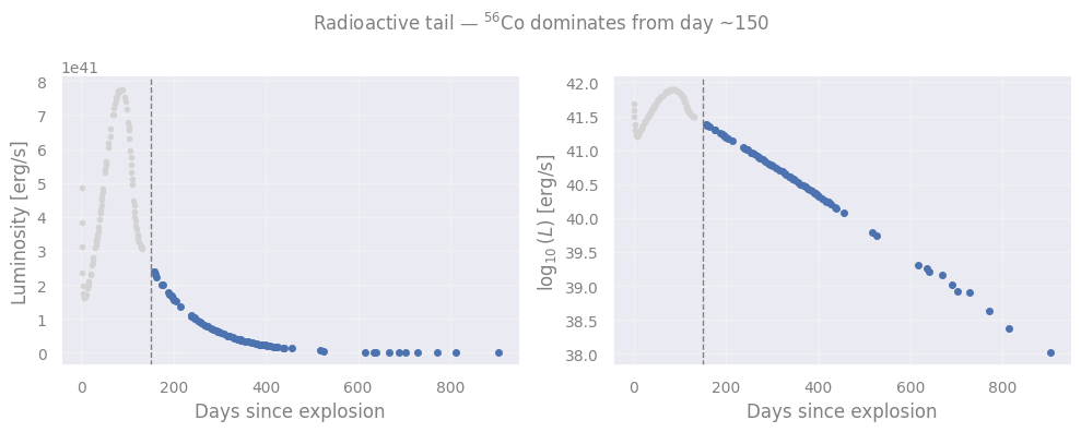
The \(^{56}\)Ni decays quickly (half-life ~6 days), so from \(t \gtrsim 130\) days the light curve is dominated entirely by \(^{56}\)Co decay, following a pure exponential:
where \(L_0\) is the luminosity extrapolated to \(t=0\) (encodes the \(^{56}\)Ni mass synthesized in the explosion) and \(\tau_{\rm Co} = 111.5\) days is the mean lifetime of \(^{56}\)Co.
Why is this non-linear? \(\tau_{\rm Co}\) appears in the exponent, and that is why we need an iterative method like Levenberg-Marquardt.
Objective: Evaluate the best-fit model to the data. But you should be careful where the fit is valid.
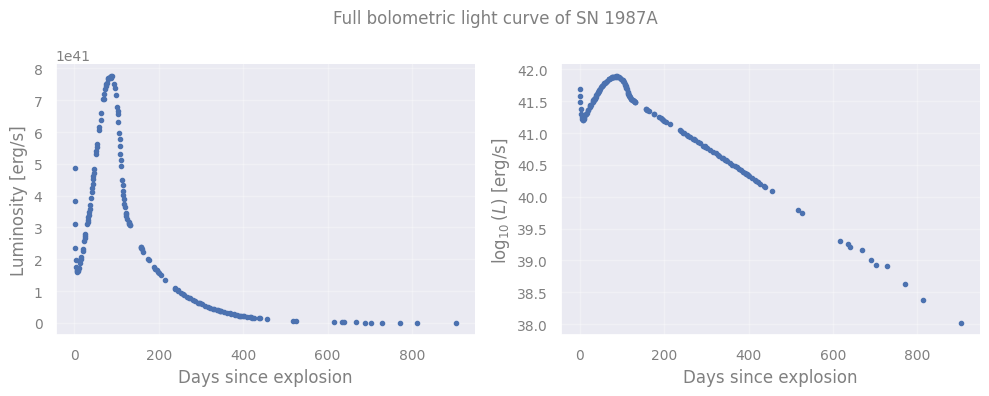
Dataset: The UVOIR bolometric light curve of SN 1987A from Suntzeff & Bouchet (1990, AJ 99, 650), Table II — the closest supernova observed in modern times (~50 kpc, Large Magellanic Cloud). 161 measurements from day 1 to day 903 since the explosion.
Tasks: In particular, you will have to:
Look at the data and define where the fit should be applied.
Define the model function
Provide physically motivated initial guesses for
L0andtau— use the log-scale plot to estimate them by eye (hint: in log scale the model is a straight line with slope \(-1/(\tau \cdot \ln 10)\);L0is the \(t=0\) extrapolation)Run the fit on the appropriate fitted range only
Plot the data and best-fit model together (log scale recommended) . Compare your recovered \(\hat{\tau}\) against the known value \(\tau_{\rm Co} = 111.5\) days — do they agree within the fit uncertainties?
Extension: Using your best-fit \(L_0\), convert it to a \(^{56}\)Ni mass using:
where \(\lambda_{\rm Co} = 1/(\tau_{\rm Co} \cdot 86400)\) s\(^{-1}\), \(\epsilon_{\rm Co} = 3.85\) MeV \(= 6.17 \times 10^{-6}\) erg per decay, \(N_A = 6.022\times10^{23}\) mol\(^{-1}\), \(A=56\) g/mol. Express in solar masses and compare with Seitenzahl et al. (2014): \(M(^{56}\text{Ni}) = 0.071 \pm 0.003\,M_\odot\).
import numpy as np
import matplotlib.pyplot as plt

data = np.loadtxt('data/SN1987A_Suntzeff1990_TableII.txt', comments='#')

time = data[:,0]
logL = data[:,1]
Lum = ...

fig, axes = plt.subplots(1, 2, figsize=(10, 4))

# plot luminosity here
axes[0].plot(... , ... , 'o', ms=3, c='C0')
axes[0].set_xlabel('Days since explosion')
axes[0].set_ylabel('Luminosity [erg/s]')

# plot logL here - to showcase linearity in log space
axes[1].plot(... , ... , 'o', ms=3, c='C0')
axes[1].set_xlabel('Days since explosion')
axes[1].set_ylabel(r'$\log_{10}(L)$ [erg/s]')

plt.suptitle('Full bolometric light curve of SN 1987A')
plt.tight_layout()
plt.show()
# Select the radioactive tail (after that many days)
mask = (time >= ... )
time_tail = time[mask]
logL_tail = logL[mask]
Lum_tail = Lum[mask]

fig, axes = plt.subplots(1, 2, figsize=(10, 4))

axes[0].plot(time[~mask], Lum[~mask], 'o', ms=3, c='lightgrey', label='Early phase (excluded)')
axes[0].plot(time_tail, Lum_tail, 'o', ms=4, c='C0', label='Radioactive tail (fit region)')
axes[0].axvline(150, ls='--', c='grey', lw=1, label='Day 150 (fit start)')
axes[0].set_xlabel('Days since explosion')
axes[0].set_ylabel('Luminosity [erg/s]')


axes[1].plot(time[~mask], logL[~mask], 'o', ms=3, c='lightgrey', label='Early phase (excluded)')
axes[1].plot(time_tail, logL_tail, 'o', ms=4, c='C0', label='Radioactive tail (fit region)')
axes[1].axvline(150, ls='--', c='grey', lw=1, label='Day 150 (fit start)')
axes[1].set_xlabel('Days since explosion')
axes[1].set_ylabel(r'$\log_{10}(L)$ [erg/s]')

plt.suptitle('Radioactive tail — $^{56}$Co dominates from day ~150')
plt.tight_layout()
plt.show()
from lmfit import Model

# 1. Model function
def decay_model( ... ):
    return ...

# 2. Initial guesses from the log-scale plot:

L0_guess  = ...
tau_guess = ...

model  = ...
result = ...

# 4. Plot
# data for model
tt = np.linspace(time_tail[0], time_tail[-1], 1000)
logL_tt = np.log10(result.eval(t=tt))

plt.plot(... , ..., 'o', ms=4, c='C0', label='Data')
plt.plot(... , ..., lw=2, c='C1', ls='--', label='Best-fit model')
plt.xlabel('Days since explosion')
plt.ylabel(r'$\log_{10}(L)$ [erg/s]')
plt.title(r'$^{56}$Co decay fit — tail region')
plt.legend()

plt.show()

# 5. Parameter comparison
L0_fit  = ...
L0_err  = ...
tau_fit = ...
tau_err = ...

print(f"\n--- Parameter comparison ---")
print(f"Recovered  tau = {tau_fit:.2f} ± {tau_err:.2f} days")
print(f"Known  tau_Co  = 111.5 days")
print(f"Difference     = {abs(tau_fit - 111.3):.2f} days  ({abs(tau_fit - 111.3)/tau_err:.1f} sigma)")
[Solution at the end!]
Chi-square (χ\(^{2}\)) fitting#
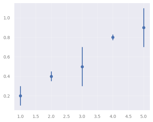
Basically, it’s least squares for when data have uncertainties on y
Instead of minimizing the sum of squares \(S(\pmb{\beta})\), we minimize the weighted average of the sum of squares, i.e., \(\chi^2\):
… where the weigths are the measurement uncertainties \(\sigma_i\).
import matplotlib.pyplot as plt

x = np.array([1, 2, 3, 4, 5])
y = np.array([0.2, 0.4, 0.5, 0.8, 0.9])
y_err = np.array([0.1, 0.05, 0.2, 0.03, 0.2])

plt.figure(figsize=(5,4))
plt.errorbar(x, y, yerr=y_err, marker="o", ls="none")
plt.show()
def linear(x, alpha, beta):
    return alpha * x + beta

model = Model(linear)

# Unweighted fit (OLS)
result_ols = model.fit(y, x=x, alpha=0.1, beta=0.1)

# Weighted fit (chi-square) — weights = 1/sigma
result_chi2 = model.fit(y, x=x, weights=1/y_err, alpha=0.1, beta=0.1)
'''
lmfit supports chi2 fitting directly via the "weights" argument. In this case we put 1/sigma_i
as the weight for each point, so that points with small errors count more and
points with large errors count less.
'''

xx = np.linspace(0.5, 5.5, 200)

plt.figure(figsize=(5, 4))
plt.errorbar(x, y, yerr=y_err, fmt='o', ms=5, capsize=4,
             color='C0', label='Data with uncertainties', zorder=3)
plt.plot(xx, result_ols.eval(x=xx),  lw=2, ls='--', color='C1',
         label=f'OLS (unweighted):  α={result_ols.params["alpha"].value:.3f}, '
               f'β={result_ols.params["beta"].value:.3f}')
plt.plot(xx, result_chi2.eval(x=xx), lw=2, color='C2',
         label=f'χ² (weighted):     α={result_chi2.params["alpha"].value:.3f}, '
               f'β={result_chi2.params["beta"].value:.3f}')
plt.xlabel('x')
plt.ylabel('y')
plt.title('OLS vs χ² weighted fit')
plt.legend(fontsize=8)
plt.tight_layout()
plt.show()

# Show which points drive the chi2 fit
print("Point weights (1/sigma):")
for xi, yi, si in zip(X, y, y_err):
    print(f"  x={xi}, y={yi}, σ={si:.2f}  →  weight={1/si:.1f}")
Point weights (1/sigma):
  x=0.0, y=0.2, σ=0.10  →  weight=10.0
  x=0.12693303650867852, y=0.4, σ=0.05  →  weight=20.0
  x=0.25386607301735703, y=0.5, σ=0.20  →  weight=5.0
  x=0.3807991095260356, y=0.8, σ=0.03  →  weight=33.3
  x=0.5077321460347141, y=0.9, σ=0.20  →  weight=5.0
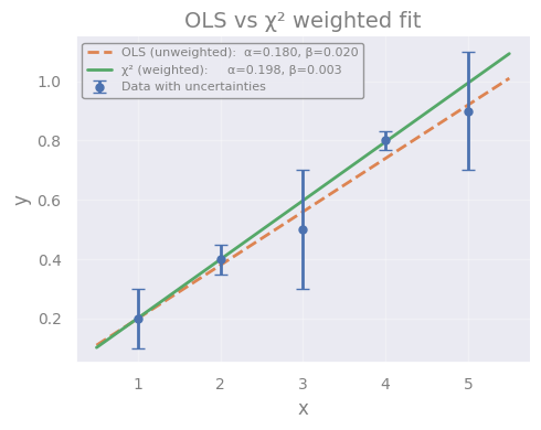
Notice how the two fits differ:
Point at \(x=2\) has \(\sigma=0.05\) → weight 20 → pulls the χ² fit strongly
Point at \(x=3\) has \(\sigma=0.20\) → weight 5 → nearly ignored by χ² fit
Point at \(x=4\) has \(\sigma=0.03\) → weight 33 → dominates the χ² fit
The χ² fit passes closer to the most precisely measured points, which is the physically correct behaviour — a measurement with a small uncertainty is more trustworthy and should constrain the model more.
When to use χ²: whenever your data points have known, unequal uncertainties — which is almost always the case in astronomy.
Further reads#
Why do we use the “reduced” \(\chi^2\) to compare model results (i.e., \(\chi_{\nu}^2\)) ? \(\rightarrow\) Andrae et al. 2010
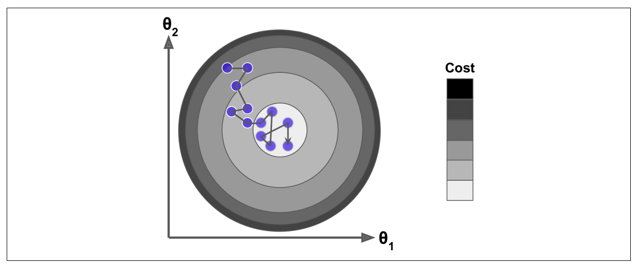
Optimization is everywhere!#
In the next lectures you will see:
MLE: Maximum Likelihood Estimation
MCMC: Markov Chain Monte Carlo
Deep Learning: Neural Network Optimization
SBI: Simulation Based Inference
… keep your mind open \(-\) you can interpret them as different flavors of optimization!
Solutions to the exercises#
Exercise 1#
from lmfit import Model

# 1. Assuming a sinusoidal model
def model_func(x, beta_1):
    y = beta_1*np.sin(x)
    return y

# 2. Using only the "_train_" data to perform the LS minimization

# Create an lmfit `Model` object:
model = Model(model_func)

# Invoking the `fit()` method, which returns the object `result`:
result = model.fit(y_train, x=X_train, beta_1=0)

# Retrieving best-fit parameters:
beta_1_hat = result.params['beta_1'].value

# 3. Calculating and plotting the model predictions on the "_train_" data
# 4. Calculating and plotting the model predictions on the "_test_" data
# Predictions of the model for train/test:
yhat_train = model_func(X_train, beta_1_hat)
yhat_test  = model_func(X_test,  beta_1_hat)

xx = np.linspace(0 ,np.max(X_test), 100)
'''Notice that `xx` is not the same as `X` (the data), but just
an array of equally spaced values that we use for plotting purposes.'''

plt.figure(figsize=(10, 4))
# Data:
plt.scatter(X_train, y_train, label='train', c='C0', s=15)
plt.scatter(X_test,  y_test,  label='test',  c='C1', s=15)
# Model:
plt.plot(xx, model_func(xx, beta_1_hat), label='model', c='grey', lw=2)
# Train predictions:
plt.scatter(X_train, yhat_train, label=r'$\hat{y}_{train}$', c='C2', s=15)
# Test predictions:
plt.scatter(X_test,  yhat_test,  label=r'$\hat{y}_{test}$',  c='C3', s=15)
#
plt.xlabel('X')
plt.ylabel('y')
plt.title('Best-fitting model')
plt.legend(loc='center left', bbox_to_anchor=(1, 0.5))
plt.show()
# 5. Calculating squares of errors for the "_train_" and "_test_":
S_train = np.sum( (yhat_train - y_train)**2 )
S_test  = np.sum( (yhat_test - y_test)**2 )

# 6. Now comparing the two squares:
print("S_train: %.2f | S_test: %.2f" % (S_train, S_test))
S_train: 0.68 | S_test: 2.43
Exercise 2#
import numpy as np
import matplotlib.pyplot as plt

data = np.loadtxt('data/SN1987A_Suntzeff1990_TableII.txt', comments='#')

time = data[:,0]
logL = data[:,1]
Lum = 10**logL


fig, axes = plt.subplots(1, 2, figsize=(10, 4))

axes[0].plot(time, Lum, 'o', ms=3, c='C0')
axes[0].set_xlabel('Days since explosion')
axes[0].set_ylabel('Luminosity [erg/s]')

axes[1].plot(time, logL, 'o', ms=3, c='C0')
axes[1].set_xlabel('Days since explosion')
axes[1].set_ylabel(r'$\log_{10}(L)$ [erg/s]')

plt.suptitle('Full bolometric light curve of SN 1987A')
plt.tight_layout()
plt.show()
# Select the radioactive tail: t >= 150 days
mask = (time >= 150)        #& (time<=400)
time_tail = time[mask]
logL_tail = logL[mask]
Lum_tail = Lum[mask]

fig, axes = plt.subplots(1, 2, figsize=(10, 4))

axes[0].plot(time[~mask], Lum[~mask], 'o', ms=3, c='lightgrey', label='Early phase (excluded)')
axes[0].plot(time_tail, Lum_tail, 'o', ms=4, c='C0', label='Radioactive tail (fit region)')
axes[0].axvline(150, ls='--', c='grey', lw=1, label='Day 150 (fit start)')
axes[0].set_xlabel('Days since explosion')
axes[0].set_ylabel('Luminosity [erg/s]')


axes[1].plot(time[~mask], logL[~mask], 'o', ms=3, c='lightgrey', label='Early phase (excluded)')
axes[1].plot(time_tail, logL_tail, 'o', ms=4, c='C0', label='Radioactive tail (fit region)')
axes[1].axvline(150, ls='--', c='grey', lw=1, label='Day 150 (fit start)')
axes[1].set_xlabel('Days since explosion')
axes[1].set_ylabel(r'$\log_{10}(L)$ [erg/s]')

plt.suptitle('Radioactive tail — $^{56}$Co dominates from day ~150')
plt.tight_layout()
plt.show()
from lmfit import Model

# 1. Model function
def decay_model(t, L0, tau):
    return L0 * np.exp(-t / tau)

# 2. Initial guesses from the log-scale plot:

#    In log scale the tail is a straight line: log10(L) = log10(L0) - t/(tau*ln10)
#    Reading off the plot: at t=200, log10(L)~41.2; at t=600, log10(L)~39.7
#    slope = (39.7 - 41.2) / (600 - 200) = -0.00375
#    => tau ~ 1 / (0.00375 * ln10) ~ 116 days  — reasonable initial guess
#    Extrapolating to t=0: intercept ~ 41.2 + 200*0.00375 = 41.95 => L0 ~ 10^41.95

L0_guess  = 10**42.0
tau_guess = 116    # days — deliberately imprecise to show LM convergence

model  = Model(decay_model)
result = model.fit(Lum_tail, t=time_tail, L0=L0_guess, tau=tau_guess)

#print(result.fit_report())

# 4. Plot
tt = np.linspace(time_tail[0], time_tail[-1], 1000)

logL_tt = np.log10(result.eval(t=tt))

plt.plot(time_tail, logL_tail, 'o', ms=4, c='C0', label='Data')
plt.plot(tt, logL_tt, lw=2, c='C1', ls='--', label='Best-fit model')
plt.xlabel('Days since explosion')
plt.ylabel(r'$\log_{10}(L)$ [erg/s]')
plt.title(r'$^{56}$Co decay fit — tail region')
plt.legend()

plt.show()

# 5. Parameter comparison
L0_fit  = result.params['L0'].value
L0_err  = result.params['L0'].stderr
tau_fit = result.params['tau'].value
tau_err = result.params['tau'].stderr

print(f"\n--- Parameter comparison ---")
print(f"Recovered  tau = {tau_fit:.2f} ± {tau_err:.2f} days")
print(f"Known  tau_Co  = 111.30 days")
print(f"Difference     = {abs(tau_fit - 111.3):.2f} days  ({abs(tau_fit - 111.5)/tau_err:.1f} sigma)")
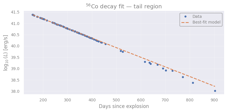
--- Parameter comparison ---
Recovered  tau = 102.19 ± 0.18 days
Known  tau_Co  = 111.30 days
Difference     = 9.11 days  (51.6 sigma)
# 6. Extension: convert L0 to 56Ni mass

M_sun      = 1.989e33      # g
N_A        = 6.022e23      # mol^-1
A          = 56.0          # g/mol
MeV_to_erg = 1.602e-6      # erg/MeV
E_decay    = 3.85          # MeV per 56Co decay
epsilon_Co = E_decay * MeV_to_erg   # erg per decay

lambda_Co  = 1.0 / (tau_fit * 86400.0)   # s^-1

# L0 = (N_Co0 / A * N_A) * lambda_Co * epsilon_Co * A/N_A
# => N_Co0 = L0 / (lambda_Co * epsilon_Co)  [atoms]
# => M_Ni  = N_Co0 * A / N_A  [grams]
N_Co0   = L0_fit / (lambda_Co * epsilon_Co)
M_Ni_g  = N_Co0 * A / N_A
M_Ni    = M_Ni_g / M_sun
M_Ni_err = (L0_err / L0_fit) * M_Ni   # dominant uncertainty from L0

print(f"Recovered M(56Ni) = {M_Ni:.4f} ± {M_Ni_err:.4f} M_sun")
print(f"Literature value  = 0.0710 ± 0.0030 M_sun  (Seitenzahl et al. 2014)")
print(f"Difference        = {abs(M_Ni - 0.071)/M_Ni_err:.1f} sigma")
Recovered M(56Ni) = 0.0747 ± 0.0003 M_sun
Literature value  = 0.0710 ± 0.0030 M_sun  (Seitenzahl et al. 2014)
Difference        = 14.1 sigma
###EOF